![]()
![]()
wakefield is designed to quickly generate random data sets. The user passes n (number of rows) and predefined vectors to the r_data_frame function to produce a dplyr::tbl_df object.
To download the development version of wakefield:
Download the zip ball or tar ball, decompress and run R CMD INSTALL on it, or use the pacman package to install the development version:
if (!require("pacman")) install.packages("pacman")
pacman::p_load_gh("trinker/wakefield")
pacman::p_load(dplyr, tidyr, ggplot2)You are welcome to:
- submit suggestions and bug-reports at: https://github.com/trinker/wakefield/issues
- send a pull request on: https://github.com/trinker/wakefield/
- compose a friendly e-mail to: tyler.rinker@gmail.com
The r_data_frame function (random data frame) takes n (the number of rows) and any number of variables (columns). These columns are typically produced from a wakefield variable function. Each of these variable functions has a pre-set behavior that produces a named vector of n length, allowing the user to lazily pass unnamed functions (optionally, without call parenthesis). The column name is hidden as a varname attribute. For example here we see the race variable function:
race(n=10)

##  [1] White White White White White White White White White White
## Levels: White Hispanic Black Asian Bi-Racial Native Other Hawaiian

attributes(race(n=10))

## $levels
## [1] "White"     "Hispanic"  "Black"     "Asian"     "Bi-Racial" "Native"
## [7] "Other"     "Hawaiian"
##
## $class
## [1] "variable" "factor"
##
## $varname
## [1] "Race"
When this variable is used inside of r_data_frame the varname is used as a column name. Additionally, the n argument is not set within variable functions but is set once in r_data_frame:
r_data_frame(
    n = 500,
    race
)

## # A tibble: 500 x 1
##    Race
##    <fct>
##  1 Hispanic
##  2 Asian
##  3 White
##  4 White
##  5 White
##  6 Black
##  7 White
##  8 Hispanic
##  9 White
## 10 Hispanic
## # ... with 490 more rows
The power of r_data_frame is apparent when we use many modular variable functions:
r_data_frame(
    n = 500,
    id,
    race,
    age,
    sex,
    hour,
    iq,
    height,
    died
)

## # A tibble: 500 x 8
##    ID    Race    Age Sex    Hour           IQ Height Died
##    <chr> <fct> <int> <fct>  <S3: times> <dbl>  <dbl> <lgl>
##  1 001   White    50 Male   00:00:00       88     68 TRUE
##  2 002   White    31 Male   00:00:00      118     72 FALSE
##  3 003   White    60 Male   00:00:00      109     68 TRUE
##  4 004   White    72 Female 00:00:00      112     68 TRUE
##  5 005   White    81 Male   00:00:00      103     71 TRUE
##  6 006   Black    21 Male   00:00:00       87     72 FALSE
##  7 007   White    64 Female 00:00:00      103     71 FALSE
##  8 008   White    26 Female 00:00:00       95     65 TRUE
##  9 009   White    41 Male   00:00:00      109     74 FALSE
## 10 010   White    64 Male   00:00:00      103     70 TRUE
## # ... with 490 more rows
There are 49 wakefield based variable functions to chose from, spanning R’s various data types (see ?variables for details).
| age | dice | hair | military | sex_inclusive |
| animal | dna | height | month | smokes |
| answer | dob | income | name | speed |
| area | dummy | internet_browser | normal | state |
| car | education | iq | political | string |
| children | employment | language | race | upper |
| coin | eye | level | religion | valid |
| color | grade | likert | sat | year |
| date_stamp | grade_level | lorem_ipsum | sentence | zip_code |
| death | group | marital | sex |
Available Variable Functions
However, the user may also pass their own vector producing functions or vectors to r_data_frame. Those with an n argument can be set by r_data_frame:
r_data_frame(
    n = 500,
    id,
    Scoring = rnorm,
    Smoker = valid,
    race,
    age,
    sex,
    hour,
    iq,
    height,
    died
)

## # A tibble: 500 x 10
##    ID    Scoring Smoker Race       Age Sex    Hour         IQ Height Died
##    <chr>   <dbl> <lgl>  <fct>    <int> <fct>  <S3: tim> <dbl>  <dbl> <lgl>
##  1 001    1.78   TRUE   White       70 Female 00:00:00     87     66 FALSE
##  2 002    1.38   TRUE   White       41 Female 00:00:00     98     61 TRUE
##  3 003    0.641  FALSE  White       81 Female 00:00:00    104     68 FALSE
##  4 004    0.461  FALSE  White       84 Female 00:00:00    109     70 TRUE
##  5 005    0.179  FALSE  White       23 Female 00:00:00    109     70 FALSE
##  6 006    0.0787 FALSE  White       32 Female 00:00:00    105     69 TRUE
##  7 007   -1.52   FALSE  White       69 Female 00:00:00    104     71 FALSE
##  8 008    1.04   FALSE  White       24 Female 00:00:00    105     74 TRUE
##  9 009   -0.390  FALSE  White       66 Female 00:00:00    103     70 FALSE
## 10 010    1.13   FALSE  Hispanic    84 Male   00:00:00     93     68 TRUE
## # ... with 490 more rows

r_data_frame(
    n = 500,
    id,
    age, age, age,
    grade, grade, grade
)

## # A tibble: 500 x 7
##    ID    Age_1 Age_2 Age_3 Grade_1 Grade_2 Grade_3
##    <chr> <int> <int> <int>   <dbl>   <dbl>   <dbl>
##  1 001      67    47    46    93.7    89.9    83.7
##  2 002      19    26    74    91.8    89      93.1
##  3 003      56    20    27    86.5    84.2    80.8
##  4 004      81    30    71    91.4    90.6    88.8
##  5 005      27    64    81    86.9    94.2    89.8
##  6 006      44    81    28    94.7    87.4    90.9
##  7 007      20    36    70    93.1    93.2    94.1
##  8 008      62    73    22    88.1    85.2    87.4
##  9 009      24    78    53    88.1    84.6    87.5
## 10 010      62    35    26    87.3    83.6    89.8
## # ... with 490 more rows
While passing variable functions to r_data_frame without call parenthesis is handy, the user may wish to set arguments. This can be done through call parenthesis as we do with data.frame or dplyr::data_frame:
r_data_frame(
    n = 500,
    id,
    Scoring = rnorm,
    Smoker = valid,
    `Reading(mins)` = rpois(lambda=20),
    race,
    age(x = 8:14),
    sex,
    hour,
    iq,
    height(mean=50, sd = 10),
    died
)

## # A tibble: 500 x 11
##    ID    Scoring Smoker `Reading(mins)` Race    Age Sex    Hour         IQ
##    <chr>   <dbl> <lgl>            <int> <fct> <int> <fct>  <S3: tim> <dbl>
##  1 001     0.900 TRUE                16 White    10 Female 00:00:00    103
##  2 002    -0.111 FALSE               19 White     9 Male   00:00:00     99
##  3 003     0.531 FALSE               16 White    13 Male   00:00:00     94
##  4 004    -1.87  FALSE               26 White     8 Female 00:00:00     83
##  5 005    -0.539 FALSE               18 White    14 Male   00:00:00    104
##  6 006    -0.646 FALSE               19 White    10 Female 00:00:00     97
##  7 007     0.326 TRUE                21 White     9 Male   00:00:00    106
##  8 008     2.34  FALSE               20 White     9 Female 00:00:00     99
##  9 009    -0.156 TRUE                27 White     8 Male   00:30:00    104
## 10 010     0.763 TRUE                17 Black    13 Female 00:30:00    108
## # ... with 490 more rows, and 2 more variables: Height <dbl>, Died <lgl>Often data contains missing values. wakefield allows the user to add a proportion of missing values per column/vector via the r_na (random NA). This works nicely within a dplyr/magrittr %>% then pipeline:
r_data_frame(
    n = 30,
    id,
    race,
    age,
    sex,
    hour,
    iq,
    height,
    died,
    Scoring = rnorm,
    Smoker = valid
) %>%
    r_na(prob=.4)

## # A tibble: 30 x 10
##    ID    Race       Age Sex    Hour         IQ Height Died  Scoring Smoker
##    <chr> <fct>    <int> <fct>  <S3: tim> <dbl>  <dbl> <lgl>   <dbl> <lgl>
##  1 01    White       81 Male   <NA>         NA     NA NA      0.862 TRUE
##  2 02    White       86 <NA>   00:30:00    109     73 TRUE   -0.274 FALSE
##  3 03    Hispanic    NA Male   03:30:00    111     65 FALSE  NA     TRUE
##  4 04    White       48 <NA>   03:30:00     NA     72 NA      0.692 TRUE
##  5 05    White       78 <NA>   03:30:00     NA     NA TRUE   NA     FALSE
##  6 06    White       80 Male   05:00:00     NA     66 NA     -0.494 TRUE
##  7 07    <NA>        NA Male   <NA>         NA     67 NA      0.861 FALSE
##  8 08    <NA>        NA Male   <NA>         88     70 TRUE   -1.76  TRUE
##  9 09    <NA>        NA Female 07:30:00     82     NA FALSE  NA     NA
## 10 10    <NA>        59 <NA>   10:00:00     90     63 TRUE    1.30  TRUE
## # ... with 20 more rowsThe r_series function allows the user to pass a single wakefield function and dictate how many columns (j) to produce.
set.seed(10)

r_series(likert, j = 3, n=10)

## # A tibble: 10 x 3
##    Likert_1       Likert_2          Likert_3
##  * <ord>          <ord>             <ord>
##  1 Neutral        Disagree          Strongly Disagree
##  2 Agree          Neutral           Disagree
##  3 Neutral        Strongly Agree    Disagree
##  4 Disagree       Neutral           Agree
##  5 Strongly Agree Agree             Neutral
##  6 Agree          Neutral           Disagree
##  7 Agree          Strongly Agree    Strongly Disagree
##  8 Agree          Agree             Agree
##  9 Disagree       Agree             Disagree
## 10 Neutral        Strongly Disagree Agree
Often the user wants a numeric score for Likert type columns and similar variables. For series with multiple factors the as_integer converts all columns to integer values. Additionally, we may want to specify column name prefixes. This can be accomplished via the variable function’s name argument. Both of these features are demonstrated here.
set.seed(10)

as_integer(r_series(likert, j = 5, n=10, name = "Item"))

## # A tibble: 10 x 5
##    Item_1 Item_2 Item_3 Item_4 Item_5
##  *  <int>  <int>  <int>  <int>  <int>
##  1      3      2      1      3      4
##  2      4      3      2      5      4
##  3      3      5      2      5      5
##  4      2      3      4      1      2
##  5      5      4      3      3      4
##  6      4      3      2      2      5
##  7      4      5      1      1      5
##  8      4      4      4      1      3
##  9      2      4      2      2      5
## 10      3      1      4      3      1
r_series can be used within a r_data_frame as well.
set.seed(10)

r_data_frame(n=100,
    id,
    age,
    sex,
    r_series(likert, 3, name = "Question")
)

## # A tibble: 100 x 6
##    ID      Age Sex    Question_1        Question_2        Question_3
##  * <chr> <int> <fct>  <ord>             <ord>             <ord>
##  1 001      54 Male   Agree             Agree             Strongly Disagr~
##  2 002      40 Male   Neutral           Strongly Agree    Disagree
##  3 003      48 Male   Disagree          Neutral           Disagree
##  4 004      67 Male   Strongly Disagree Neutral           Disagree
##  5 005      24 Female Strongly Agree    Strongly Disagree Strongly Disagr~
##  6 006      34 Female Disagree          Disagree          Agree
##  7 007      37 Female Disagree          Strongly Agree    Strongly Disagr~
##  8 008      37 Male   Strongly Disagree Agree             Agree
##  9 009      62 Female Agree             Strongly Agree    Strongly Agree
## 10 010      48 Male   Strongly Disagree Strongly Disagree Agree
## # ... with 90 more rows

set.seed(10)

r_data_frame(n=100,
    id,
    age,
    sex,
    r_series(likert, 5, name = "Item", integer = TRUE)
)

## # A tibble: 100 x 8
##    ID      Age Sex    Item_1 Item_2 Item_3 Item_4 Item_5
##  * <chr> <int> <fct>   <int>  <int>  <int>  <int>  <int>
##  1 001      54 Male        4      4      1      1      1
##  2 002      40 Male        3      5      2      1      2
##  3 003      48 Male        2      3      2      1      2
##  4 004      67 Male        1      3      2      4      3
##  5 005      24 Female      5      1      1      5      4
##  6 006      34 Female      2      2      4      3      4
##  7 007      37 Female      2      5      1      5      2
##  8 008      37 Male        1      4      4      5      5
##  9 009      62 Female      4      5      5      4      3
## 10 010      48 Male        1      1      4      1      2
## # ... with 90 more rowsThe user can also create related series via the relate argument in r_series. It allows the user to specify the relationship between columns. relate may be a named list of or a short hand string of the form of "fM_sd" where:
f is one of (+, -, *, /)M is a mean valuesd is a standard deviation of the mean valueFor example you may use relate = "*4_1". If relate = NULL no relationship is generated between columns. I will use the short hand string form here.
r_series(grade, j = 5, n = 100, relate = "+1_6")

## # A tibble: 100 x 5
##    Grade_1 Grade_2 Grade_3 Grade_4 Grade_5
##  *   <dbl>   <dbl>   <dbl>   <dbl>   <dbl>
##  1    84.5    92.5    91.6    87.4    76.7
##  2    93.1    85      81.8    87.8    91.3
##  3    81.6    67.5    52.6    48.8    56.8
##  4    92.5    89.3    95.3   102.     94.5
##  5    96.6    95.9    98.7   116.    115.
##  6    89.7    88.1    88.8    89.     86.4
##  7    92.8    91.7    98.3    98.7   102.
##  8    92.1    92.9    92.6    85.5    93.1
##  9    90.6    96.9   104.    108.    106.
## 10    96      94.8    84.3    91.1   107.
## # ... with 90 more rows

r_series(age, 5, 100, relate = "+5_0")

## # A tibble: 100 x 5
##    Age_1 Age_2 Age_3 Age_4 Age_5
##  * <dbl> <dbl> <dbl> <dbl> <dbl>
##  1    37    42    47    52    57
##  2    37    42    47    52    57
##  3    51    56    61    66    71
##  4    29    34    39    44    49
##  5    72    77    82    87    92
##  6    50    55    60    65    70
##  7    23    28    33    38    43
##  8    59    64    69    74    79
##  9    85    90    95   100   105
## 10    77    82    87    92    97
## # ... with 90 more rows

r_series(likert, 5,  100, name ="Item", relate = "-.5_.1")

## # A tibble: 100 x 5
##    Item_1 Item_2 Item_3 Item_4 Item_5
##  *  <dbl>  <dbl>  <dbl>  <dbl>  <dbl>
##  1      2      1      0     -1     -1
##  2      3      2      1      1      0
##  3      1      1      1      0      0
##  4      4      3      3      2      1
##  5      2      1      1      0      0
##  6      2      1      1      1      0
##  7      1      0      0     -1     -2
##  8      2      2      1      1      0
##  9      2      2      1      0      0
## 10      3      3      3      3      3
## # ... with 90 more rows

r_series(grade, j = 5, n = 100, relate = "*1.05_.1")

## # A tibble: 100 x 5
##    Grade_1 Grade_2 Grade_3 Grade_4 Grade_5
##  *   <dbl>   <dbl>   <dbl>   <dbl>   <dbl>
##  1    85.7    94.3   113.    113.    113.
##  2    86.4    77.8    77.8    85.5    85.5
##  3    90.6    99.7    89.7    98.7   109.
##  4    89.1    89.1    89.1    71.3    71.3
##  5    87      95.7   115.    103.    114.
##  6    93.9   103.    124.    136.    136.
##  7    80.1    72.1    64.9    84.3    84.3
##  8    91.7   110.    132.    132.    145.
##  9    87.4    96.1    96.1   106.    116.
## 10    92.9    92.9    83.6    92.0   101.
## # ... with 90 more rowsUse the sd command to adjust correlations.
round(cor(r_series(grade, 8, 10, relate = "+1_2")), 2)

##         Grade_1 Grade_2 Grade_3 Grade_4 Grade_5 Grade_6 Grade_7 Grade_8
## Grade_1    1.00    0.85    0.64    0.39    0.28    0.25    0.28    0.15
## Grade_2    0.85    1.00    0.86    0.68    0.61    0.56    0.56    0.47
## Grade_3    0.64    0.86    1.00    0.77    0.70    0.80    0.86    0.78
## Grade_4    0.39    0.68    0.77    1.00    0.94    0.80    0.65    0.74
## Grade_5    0.28    0.61    0.70    0.94    1.00    0.85    0.69    0.73
## Grade_6    0.25    0.56    0.80    0.80    0.85    1.00    0.92    0.89
## Grade_7    0.28    0.56    0.86    0.65    0.69    0.92    1.00    0.91
## Grade_8    0.15    0.47    0.78    0.74    0.73    0.89    0.91    1.00

round(cor(r_series(grade, 8, 10, relate = "+1_0")), 2)

##         Grade_1 Grade_2 Grade_3 Grade_4 Grade_5 Grade_6 Grade_7 Grade_8
## Grade_1       1       1       1       1       1       1       1       1
## Grade_2       1       1       1       1       1       1       1       1
## Grade_3       1       1       1       1       1       1       1       1
## Grade_4       1       1       1       1       1       1       1       1
## Grade_5       1       1       1       1       1       1       1       1
## Grade_6       1       1       1       1       1       1       1       1
## Grade_7       1       1       1       1       1       1       1       1
## Grade_8       1       1       1       1       1       1       1       1

round(cor(r_series(grade, 8, 10, relate = "+1_20")), 2)

##         Grade_1 Grade_2 Grade_3 Grade_4 Grade_5 Grade_6 Grade_7 Grade_8
## Grade_1    1.00    0.26    0.27    0.40    0.21   -0.21   -0.36   -0.41
## Grade_2    0.26    1.00    0.77    0.60    0.64    0.50    0.53    0.46
## Grade_3    0.27    0.77    1.00    0.78    0.76    0.66    0.62    0.66
## Grade_4    0.40    0.60    0.78    1.00    0.95    0.76    0.59    0.55
## Grade_5    0.21    0.64    0.76    0.95    1.00    0.82    0.65    0.61
## Grade_6   -0.21    0.50    0.66    0.76    0.82    1.00    0.90    0.82
## Grade_7   -0.36    0.53    0.62    0.59    0.65    0.90    1.00    0.94
## Grade_8   -0.41    0.46    0.66    0.55    0.61    0.82    0.94    1.00

round(cor(r_series(grade, 8, 10, relate = "+15_20")), 2)

##         Grade_1 Grade_2 Grade_3 Grade_4 Grade_5 Grade_6 Grade_7 Grade_8
## Grade_1    1.00   -0.10   -0.50   -0.39   -0.25   -0.52   -0.26   -0.31
## Grade_2   -0.10    1.00    0.74    0.50    0.13    0.03    0.36    0.46
## Grade_3   -0.50    0.74    1.00    0.81    0.48    0.41    0.71    0.78
## Grade_4   -0.39    0.50    0.81    1.00    0.75    0.66    0.58    0.75
## Grade_5   -0.25    0.13    0.48    0.75    1.00    0.91    0.70    0.74
## Grade_6   -0.52    0.03    0.41    0.66    0.91    1.00    0.58    0.57
## Grade_7   -0.26    0.36    0.71    0.58    0.70    0.58    1.00    0.78
## Grade_8 -0.31 0.46 0.78 0.75 0.74 0.57 0.78 1.00dat <- r_data_frame(12,
name,
r_series(grade, 100, relate = "+1_6")
)
dat %>%
gather(Time, Grade, -c(Name)) %>%
mutate(Time = as.numeric(gsub("\\D", "", Time))) %>%
ggplot(aes(x = Time, y = Grade, color = Name, group = Name)) +
geom_line(size=.8) +
theme_bw()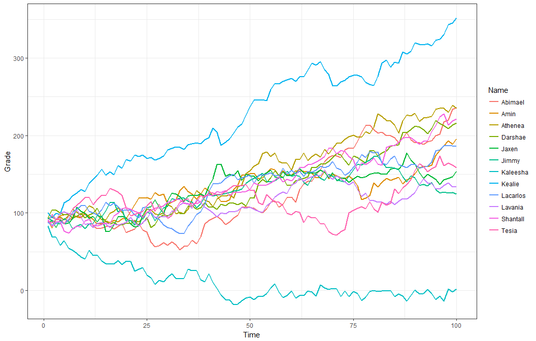
The user may wish to expand a factor into j dummy coded columns. The r_dummy function expands a factor into j columns and works similar to the r_series function. The user may wish to use the original factor name as the prefix to the j columns. Setting prefix = TRUE within r_dummy accomplishes this.
set.seed(10)
r_data_frame(n=100,
    id,
    age,
    r_dummy(sex, prefix = TRUE),
    r_dummy(political)
)

## # A tibble: 100 x 9
##    ID      Age Sex_Male Sex_Female Democrat Republican Constitution
##  * <chr> <int>    <int>      <int>    <int>      <int>        <int>
##  1 001      54        1          0        1          0            0
##  2 002      40        1          0        1          0            0
##  3 003      48        1          0        0          1            0
##  4 004      67        1          0        0          1            0
##  5 005      24        0          1        1          0            0
##  6 006      34        0          1        0          1            0
##  7 007      37        0          1        0          1            0
##  8 008      37        1          0        0          0            0
##  9 009      62        0          1        1          0            0
## 10 010      48        1          0        0          1            0
## # ... with 90 more rows, and 2 more variables: Libertarian <int>,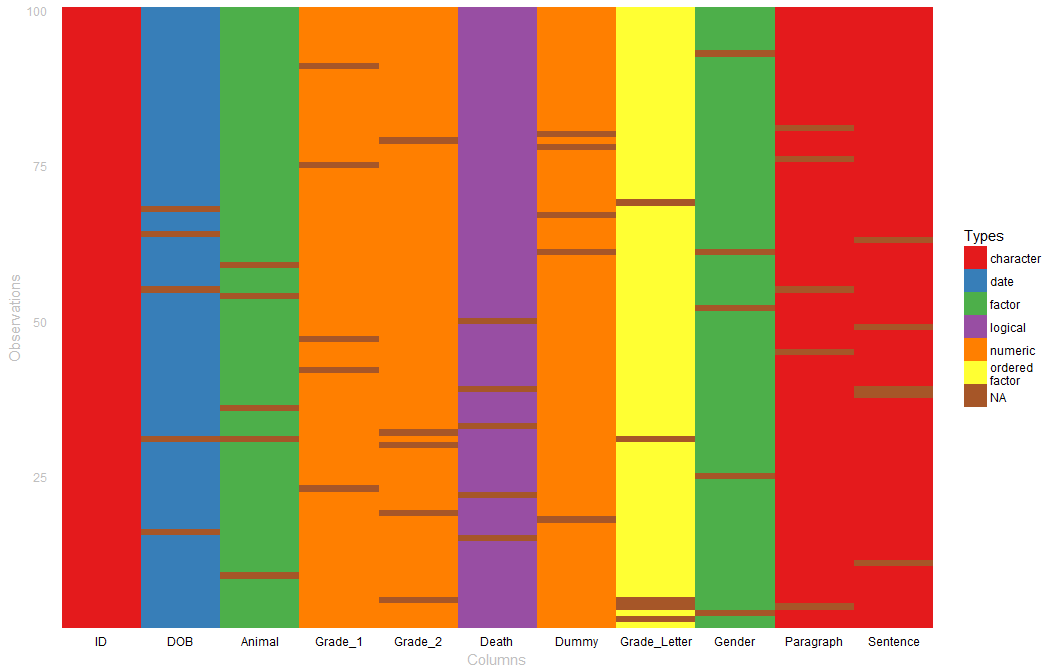
## # Green <int>It is helpful to see the column types and NAs as a visualization. The table_heat (also the plot method assigned to tbl_df as well) can provide visual glimpse of data types and missing cells.
set.seed(10)

r_data_frame(n=100,
    id,
    dob,
    animal,
    grade, grade,
    death,
    dummy,
    grade_letter,
    gender,
    paragraph,
    sentence
) %>%
   r_na() %>%
   plot(palette = "Set1")