README

An R-package which contains functions to set up risk-adjusted quality control charts in health care.

Main features

Installation

install.packages("vlad")

# install.packages("devtools")
devtools::install_github("wittenberg/vlad")

Example

library("vlad")
library("dplyr")
library("tidyr")
library("ggplot2")

Subset the dataset cardiacsurgery into Phase I (first two years) and Phase II (five years) and estimate a risk model based on phaseI.

data("cardiacsurgery", package = "spcadjust")
cardiacsurgery <- cardiacsurgery %>% rename(s = Parsonnet) %>%
  mutate(y = ifelse(status == 1 & time <= 30, 1, 0),
        phase = factor(ifelse(date < 2*365, "I", "II")))
head(cardiacsurgery)
#>   date time status  s surgeon y phase
#> 1    1   90      0 15       7 0     I
#> 2    1   90      0  9       3 0     I
#> 3    2   90      0  2       5 0     I
#> 4    3   90      0  8       7 0     I
#> 5    3   90      0  7       1 0     I
#> 6    3   90      0 40       1 0     I
phaseI <- filter(cardiacsurgery, phase == "I") %>% select(s, y)
coeff <- round(coef(glm(y ~ s, data = phaseI, family = "binomial")), 3)
print(coeff)
#> (Intercept)           s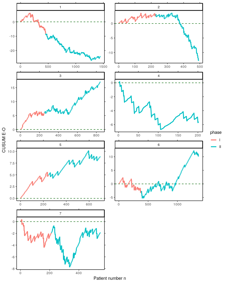 
#>       -3.79        0.08

Create VLADs for seven surgeons

By using the estimated risk model coefficients coeff, for each pair of Parsonnet score s and operation outcome values y, the difference between expected and observed outcome is calculated with the function calceo(). Thereafter, differences are cummulated to create the VLAD. This is done for all seven surgeons of the cardiacsurgery dataset. Results are saved to the object vlads7.

vlads7 <- lapply(1:7, function(j){
  Si <- filter(cardiacsurgery, surgeon == j)
  EO <- sapply(seq_along(Si$s), function(i) calceo(df = Si[i, c("s", "y")], coeff = coeff))
  select(Si, surgeon, phase) %>%  mutate(n = 1:length(EO), cEO = cumsum(EO))
})

Create Variable life-adjusted Displays for each surgeon from the object vlads7.

vlads7 %>% 
  bind_rows() %>%  
  gather(key = "Surgeon", value = value, c(-n, -surgeon, -phase)) %>%
  ggplot(aes(x = n, y = value, colour = phase, group = Surgeon)) +
    geom_hline(yintercept = 0, colour = "darkgreen", linetype = "dashed") +
    geom_line(size = 1.1) + facet_wrap( ~ surgeon, ncol = 2, scales = "free") +
    labs(x="Patient number n", y="CUSUM E-O") + theme_classic() +
    scale_y_continuous(sec.axis = dup_axis(name = NULL, labels = NULL)) +
    scale_x_continuous(sec.axis = dup_axis(name = NULL, labels = NULL))

Create a VLAD for surgeon 2

S2 <- filter(cardiacsurgery, surgeon == 2) %>% select(phase, s, y)
S2I <- subset(S2, c(phase == "I"))
S2II <- subset(S2, c(phase == "II"))
coeff <- coef(glm(y ~ s, data = S2I, family = "binomial"))
EO <- sapply(1:nrow(S2), function(i) calceo(df = S2[i, c("s", "y")], coeff = coeff))

df1 <- select(S2, phase) %>% mutate(n = row_number(), cEO = cumsum(EO))
df2 <- gather(df1, variable, value, c(-n, -phase))

p1 <- ggplot(df2, aes(x = n, y = value, colour = phase)) +
  geom_hline(yintercept = 0, linetype = "dashed") + geom_line() + geom_point() + 
  labs(x = "Patient number", y = "CUSUM E-O") + theme_classic() +
  scale_y_continuous(sec.axis = dup_axis(name = NULL, labels = NULL)) +
  scale_x_continuous(sec.axis = dup_axis(name = NULL, labels = NULL))
p1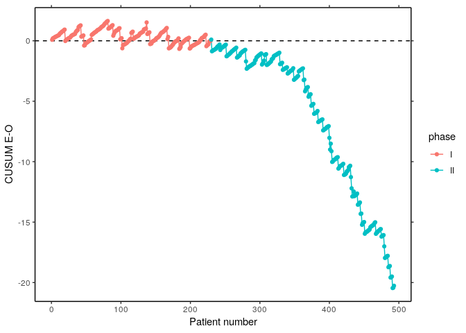

Compute thresholds of a risk-adjusted CUSUM chart for surgeon 2

Upper and lower control limits of the risk-adjusted CUSUM chart based on log-likelihood ratio statistic can be computed with the function racusum_arl_h_sim(). The implemention uses parallel simulation and a multi-stage search procedure.

# set a random number generator for parallel computations
RNGkind("L'Ecuyer-CMRG")
# number of simulation runs
m <- 10^4
# assign cores
nc <- parallel::detectCores()
# verbose calculation 
UCL_sim <- racusum_crit_sim(L0 = 740, df = S2I[, c("s", "y")], coeff = coeff, m = m, RA = 2, nc = nc, verbose = TRUE)
#> h = 1    ARL = 75.006 
#> h = 2    ARL = 383.3554 
#> h = 3    ARL = 1312.8564 
#> h = 2.9  ARL = 1181.3768 
#> h = 2.8  ARL = 1052.3355 
#> h = 2.7  ARL = 928.6587 
#> h = 2.6  ARL = 822.3063 
#> h = 2.5  ARL = 730.0184 
#> h = 2.51     ARL = 739.8392 
#> h = 2.52     ARL = 747.3412 
#> h = 2.519    ARL = 746.4942 
#> h = 2.518    ARL = 745.9933 
#> h = 2.517    ARL = 745.6282 
#> h = 2.516    ARL = 744.6935 
#> h = 2.515    ARL = 744.0614 
#> h = 2.514    ARL = 743.2221 
#> h = 2.513    ARL = 742.2656 
#> h = 2.512    ARL = 741.7172 
#> h = 2.511    ARL = 741.3188 
#> h = 2.51     ARL = 739.8392 
#> h = 2.5101   ARL = 739.862 
#> h = 2.5102   ARL = 739.862 
#> h = 2.5103   ARL = 740.0315
# quite calculation
LCL_sim <- racusum_crit_sim(L0 = 740, df = S2I[, c("s", "y")], coeff = coeff, m = m, RA = 1/2, nc = nc, verbose = FALSE)
round(cbind(UCL_sim, LCL_sim), 3)
#>      UCL_sim LCL_sim
#> [1,]    2.51   2.281

vlad

Main features

Installation

Example

Create VLADs for seven surgeons

Create a VLAD for surgeon 2

Compute thresholds of a risk-adjusted CUSUM chart for surgeon 2

References

Authors

License