


tidyBF: Tidy Wrapper for BayesFactor Package![]()
![]()
![]()
![]()
![]()
![]()
tidyBF package is a tidy wrapper around the BayesFactor package that always expects the data to be in the tidy format and return a tibble containing Bayes Factor values. Additionally, it provides a more consistent syntax and by default returns a dataframe with rich details. These functions can also return expressions containing results from Bayes Factor tests that can then be displayed in custom plots.
To get the latest, stable CRAN release:
You can get the development version of the package from GitHub. To see what new changes (and bug fixes) have been made to the package since the last release on CRAN, you can check the detailed log of changes here: https://indrajeetpatil.github.io/tidyBF/news/index.html
If you are in hurry and want to reduce the time of installation, prefer-
# needed package to download from GitHub repo
install.packages("remotes")

remotes::install_github(
  repo = "IndrajeetPatil/tidyBF", # package path on GitHub
  quick = TRUE # skips docs, demos, and vignettes
)
If time is not a constraint-
remotes::install_github(
  repo = "IndrajeetPatil/tidyBF", # package path on GitHub
  dependencies = TRUE, # installs packages which `tidyBF` depends on
  upgrade_dependencies = TRUE # updates any out of date dependencies
)Below are few concrete examples of where tidyBF wrapper might provide a more friendly way to access output from or write functions around BayesFactor.
BayesFactor is inconsistent with its formula interface. tidyBF avoids this as it doesn’t provide the formula interface for any of the functions.
# setup
set.seed(123)

# with `BayesFactor` ----------------------------------------
suppressPackageStartupMessages(library(BayesFactor))
data(sleep)

# independent t-test: accepts formula interface
ttestBF(formula = wt ~ am, data = mtcars)
#> Bayes factor analysis
#> --------------
#> [1] Alt., r=0.707 : 1383.367 ±0%
#>
#> Against denominator:
#>   Null, mu1-mu2 = 0
#> ---
#> Bayes factor type: BFindepSample, JZS

# paired t-test: doesn't accept formula interface
ttestBF(formula = extra ~ group, data = sleep, paired = TRUE)
#> Error in ttestBF(formula = extra ~ group, data = sleep, paired = TRUE): Cannot use 'paired' with formula.

# with `tidyBF` ----------------------------------------
library(tidyBF)

# independent t-test
bf_ttest(data = mtcars, x = am, y = wt)
#> # A tibble: 1 x 7
#>    bf10     bf01 log_e_bf10 log_e_bf01 log_10_bf10 log_10_bf01 bf.prior
#>   <dbl>    <dbl>      <dbl>      <dbl>       <dbl>       <dbl>    <dbl>
#> 1 1383. 0.000723       7.23      -7.23        3.14       -3.14    0.707

# paired t-test
bf_ttest(data = sleep, x = group, y = extra, paired = TRUE)
#> # A tibble: 1 x 7
#>    bf10   bf01 log_e_bf10 log_e_bf01 log_10_bf10 log_10_bf01 bf.prior
#>   <dbl>  <dbl>      <dbl>      <dbl>       <dbl>       <dbl>    <dbl>
#> 1 17.3 0.0579 2.85 -2.85 1.24 -1.24 0.707Although all functions default to returning a dataframe, you can also use it to extract expressions that can be displayed in plots.
# setup
set.seed(123)
library(ggplot2)

# using the expression to display details in a plot
ggplot(ToothGrowth, aes(supp, len)) +
  geom_boxplot() + # two-sample t-test results in an expression
  labs(subtitle = bf_ttest(ToothGrowth, supp, len, output = "alternative"))
Here is another example:
# setup
set.seed(123)
library(ggplot2)

# using the expression to display details in a plot
ggplot(mtcars, aes(wt, mpg)) + # Pearson's r results in an expression
  geom_point() + geom_smooth(method = "lm") +
  labs(subtitle = bf_corr_test(mtcars, wt, mpg, output = "null"))
#> `geom_smooth()` using formula 'y ~ x'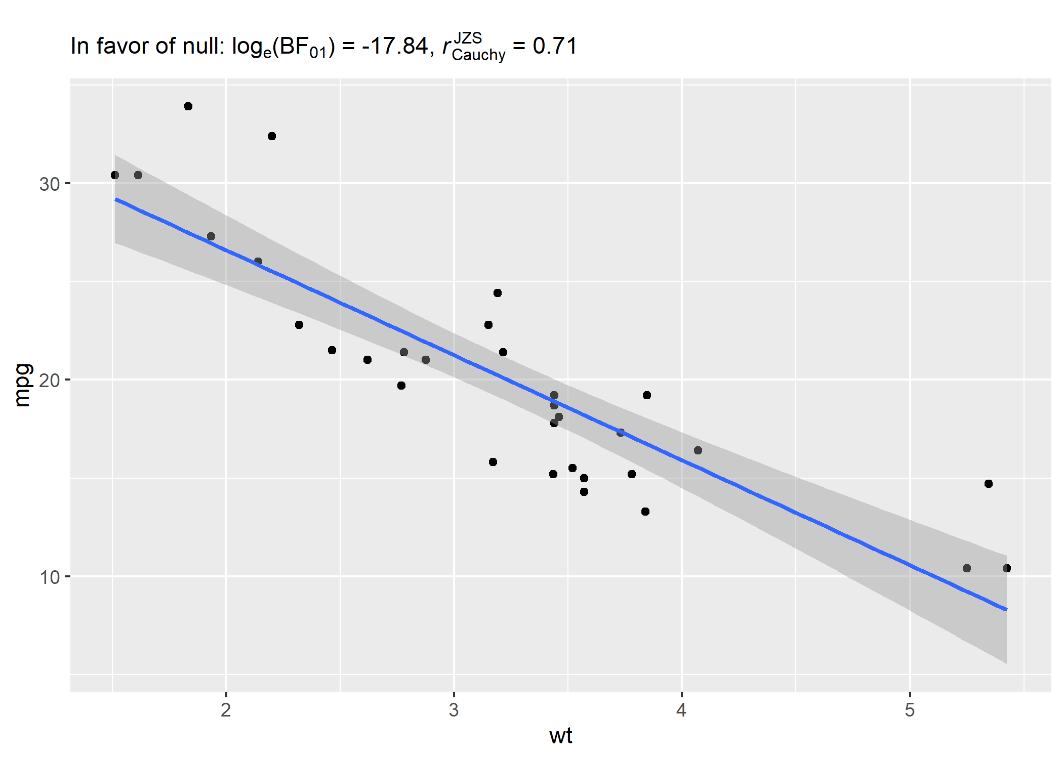
BayesFactor can return the Bayes Factor value corresponding to either evidence in favor of the null hypothesis over the alternative hypothesis (BF01) or in favor of the alternative over the null (BF10), depending on how this object is called. tidyBF on the other hand return both of these values and their logarithms.
# `BayesFactor` object
bf <- BayesFactor::correlationBF(y = iris$Sepal.Length, x = iris$Petal.Length)

# alternative
bf
#> Bayes factor analysis
#> --------------
#> [1] Alt., r=0.333 : 2.136483e+43 ±0%
#>
#> Against denominator:
#>   Null, rho = 0
#> ---
#> Bayes factor type: BFcorrelation, Jeffreys-beta*

# null
1 / bf
#> Bayes factor analysis
#> --------------
#> [1] Null, rho = 0 : 4.680589e-44 ±0%
#>
#> Against denominator:
#>   Alternative, r = 0.333333333333333, rho =/= 0
#> ---
#> Bayes factor type: BFcorrelation, Jeffreys-beta*

# `tidyBF` output
bf_corr_test(iris, Sepal.Length, Petal.Length, bf.prior = 0.333)
#> # A tibble: 1 x 7
#>      bf10     bf01 log_e_bf10 log_e_bf01 log_10_bf10 log_10_bf01 bf.prior
#>     <dbl>    <dbl>      <dbl>      <dbl>       <dbl>       <dbl>    <dbl>
#> 1 2.13e43 4.70e-44       99.8      -99.8        43.3       -43.3    0.333
Note that the log-transformed values are helpful because in case of strong effects, the raw Bayes Factor values can be pretty large, but the log-transformed values continue to remain easy to work with.
The hexsticker was generously designed by Sarah Otterstetter (Max Planck Institute for Human Development, Berlin).
Please note that the tidyBF project is released with a Contributor Code of Conduct. By contributing to this project, you agree to abide by its terms.