

Recursive functions are the natural way to express iterations in a functional programming langauge, but in R, they can be significantly slower than loop-versions and for moderately long sequences or moderately deep trees, recursive functions will reach a limit imposted on them by the stack limit.
There are known solutions to these problems, as long as functions are written to be tail-recursive, meaning that the return value of a function is either a base value or another recursive call, but where we do not call recursively to then do something with the result.
The goal of tailr is to automatically transform tail-recursive functions into loops or trampolines.
You can install the released version of tailr from CRAN using
You can install tailr from GitHub with:
Consider a classical recursive function, factorial:
(I know R already has a builtin factorial function, but please ignore that). This function will compute the factorial of n, but if n is too large, it will exceed the stack limit:
A classical way out of this problem is to turn it into a tail-recursive function:
R doesn’t implement the tail-recursion optimisation, though, so it doesn’t help us.
With tailr we can, automatically, translate a tail-recursive function into a looping one, essentially implementing the tail-recursion optimisation this way.
I have disabled byte compilation to make running time comparisons fair below; by default it is enabled. For a function as simple as factorial, though, byte compiling will not affect the running time in any substantial amount.
This version, because it looks instead of recurse, doesn’t have the stack limit problem:
We get the result Inf because the number we compute is too large to represent on the computer, but that is not the point of the example. The point is that the recursion doesn’t get too deep for the stack because we avoid recursion alltogether.
With something as simple as computing the factorial, it is easy to write a looping function by hand, and it will be much faster than both the (tail-)recursive and the transformed function:
loop_factorial <- function(n) {
    val <- 1
    while (n > 1) {
        val <- n * val
        n <- n - 1
    }
    val
}


n <- 1000
bm <- microbenchmark::microbenchmark(factorial(n),
                                     tr_factorial(n),
                                     loop_factorial(n))
bm
#> Unit: microseconds
#>               expr     min       lq      mean   median       uq      max
#>       factorial(n) 699.833 790.4000 994.13872 856.2115 1076.836 5492.965
#>    tr_factorial(n) 780.342 803.4845 939.39344 838.3140 1047.651 2804.756
#>  loop_factorial(n)  57.173  59.7730  85.75384  60.6195   61.887 2359.777
#>  neval
#>    100
#>    100
#>    100
boxplot(bm)
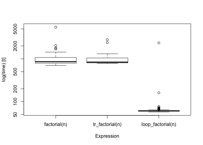
The transformed version runs in about the same time as the recursive one, but the looping function is much faster.
However, consider a more complicated example. Using the pmatch package, we can create a linked list data structure as this:
A natural way to process linked lists using pattern matching is to write recursive functions that matches different patterns of their input. A function for computing the length of a linked list can look like this:
The function we generate is rather complicated
body(tr_llength)
#> .Primitive("{")(.tailr_.match_expr <- .match_expr, .tailr_acc <- acc,
#>     callCC(function(escape) {
#>         repeat {
#>             .Primitive("{")(.match_expr <- .tailr_.match_expr,
#>                 acc <- .tailr_acc, if (is.na(.match_expr) &&
#>                   attr(.match_expr, "constructor") == "NIL")
#>                   escape(acc)
#>                 else if ({
#>                   .cons <- attr(.match_expr, "constructor")
#>                   !is.null(.cons) && .cons == "CONS"
#>                 } && {
#>                   car <- .match_expr$car
#>                   TRUE
#>                 } && {
#>                   cdr <- .match_expr$cdr
#>                   TRUE
#>                 }) {
#>                   .tailr_.match_expr <<- cdr
#>                   .tailr_acc <<- acc + 1
#>                 }
#>                 else {
#>                   escape(stop("None of the patterns match."))
#>                 }, next)
#>         }
#>     }))
but, then, it is not one we want to manually inspect in any case.
It is not too hard to implement this function with a loop either, but it is not as simple as the recursive function:
is_nil <- case_func(NIL -> TRUE, otherwise -> FALSE)
loop_llength <- function(llist) {
    len <- 0
    while (!is_nil(llist)) {
        len <- len + 1
        llist <- llist$cdr
    }
    len
}
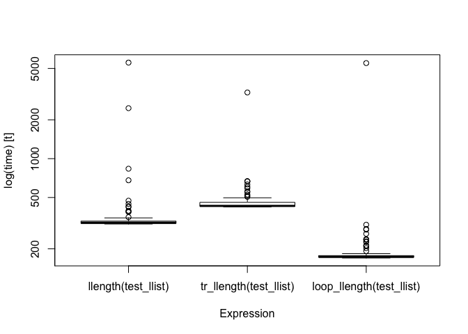
If we compare the running time for these three functions, the transformed function is faster than the recursive but not as fast as the iterative:
make_llist <- function(n) {
    l <- NIL
    for (i in 1:n) {
        l <- CONS(i, l)
    }
    l
}
test_llist <- make_llist(100)
bm <- microbenchmark::microbenchmark(llength(test_llist),
                                     tr_llength(test_llist),
                                     loop_llength(test_llist))
bm
#> Unit: microseconds
#>                      expr     min      lq     mean   median       uq
#>       llength(test_llist) 311.461 314.529 410.0324 318.8050 327.9455
#>    tr_llength(test_llist) 422.970 426.982 481.7691 430.3400 458.4060
#>  loop_llength(test_llist) 169.677 171.921 235.7967 173.4075 177.2230
#>       max neval
#>  5551.296   100
#>  3257.986   100
#>  5502.246   100
boxplot(bm)
FIXME: The main reason for this is that the running time is dominated by the cost of pmatch. If I manage to get that faster, the iterative function might end being much faster here as well.
More examples:
llcontains <- case_func(x,
    NIL -> FALSE,
    CONS(car, cdr) -> if (car == x) TRUE else llcontains(cdr, x)
)

tr_llcontains <- tailr::loop_transform(llcontains)

loop_contains <- function(lst, x) {
    while (!is_nil(lst)) {
        if (x == lst$car) return(TRUE)
        else lst <- lst$cdr
    }
}

lst <- make_llist(100)
bm <- microbenchmark::microbenchmark(llcontains(lst, 1001),
                                     tr_llcontains(lst, 1001),
                                     loop_contains(lst, 1001))
bm
#> Unit: microseconds
#>                      expr     min       lq     mean   median       uq
#>     llcontains(lst, 1001) 308.417 320.6750 461.6773 335.1845 376.4935
#>  tr_llcontains(lst, 1001) 432.907 448.2985 509.1565 469.4505 504.8375
#>  loop_contains(lst, 1001) 235.567 241.9755 306.6966 258.8265 286.5830
#>       max neval
#>  5073.269   100
#>  2596.863   100
#>  2548.667   100
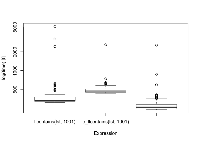
boxplot(bm)
llrev <- pmatch::case_func(acc = NIL,
    NIL -> acc,
    CONS(car, cdr) -> llrev(cdr, CONS(car, acc))
)

bubble <- case_func(swapped = FALSE, acc = NIL,
    CONS(first, CONS(second, rest)) ->
        if (first > second) bubble(CONS(first, rest), TRUE, CONS(second, acc))
        else bubble(CONS(second, rest), swapped, CONS(first, acc)),
    CONS(x, NIL) -> list(new_list = llrev(CONS(x, acc)), swapped = swapped)
)

bubble_sort <- function(lst) {
    if (is_nil(lst)) return(lst)
    bind[lst, swapped] <- bubble(lst)
    while (swapped) {
        bind[lst, swapped] <- bubble(lst)
    }
    lst
}

lst <- CONS(3, CONS(2, CONS(5, CONS(1, NIL))))
bubble_sort(lst)
#> CONS(car = 1, cdr = CONS(car = 2, cdr = CONS(car = 3, cdr = CONS(car = 5, cdr = NIL))))
tr_llrev <- pmatch::case_func(acc = NIL,
NIL -> acc,
CONS(car, cdr) -> llrev(cdr, CONS(car, acc))
)
tr_llrev <- tailr::loop_transform(tr_llrev)
tr_bubble <- case_func(swapped = FALSE, acc = NIL,
CONS(first, CONS(second, rest)) ->
if (first > second) tr_bubble(CONS(first, rest), TRUE, CONS(second, acc))
else tr_bubble(CONS(second, rest), swapped, CONS(first, acc)),
CONS(x, NIL) -> list(new_list = tr_llrev(CONS(x, acc)), swapped = swapped)
)
tr_bubble <- tailr::loop_transform(tr_bubble)
tr_bubble_sort <- function(lst) {
if (is_nil(lst)) return(lst)
bind[lst, swapped] <- tr_bubble(lst)
while (swapped) {
bind[lst, swapped] <- tr_bubble(lst)
}
lst
}
lst <- CONS(3, CONS(2, CONS(5, CONS(1, NIL))))
tr_bubble_sort(lst)
#> CONS(car = 1, cdr = CONS(car = 2, cdr = CONS(car = 3, cdr = CONS(car = 5, cdr = NIL))))loop_llrev <- function(lst) {
acc <- NIL
while (!is_nil(lst)) {
acc <- CONS(lst$car, acc)
lst <- lst$cdr
}
acc
}
loop_bubble <- function(lst, swapped = FALSE) {
acc <- NIL
repeat {
if (is_nil(lst$cdr))
return(list(new_list = loop_llrev(CONS(lst$car, acc)),
swapped = swapped))
first <- lst$car
second <- lst$cdr$car
rest <- lst$cdr$cdr
if (first > second) {
acc <- CONS(second, acc)
lst <- CONS(first, rest)
swapped <- TRUE
} else {
acc <- CONS(first, acc)
lst <- CONS(second, rest)
}
}
}
loop_bubble_sort <- function(lst) {
if (is_nil(lst)) return(lst)
bind[lst, swapped] <- loop_bubble(lst)
while (swapped) {
bind[lst, swapped] <- loop_bubble(lst)
}
lst
}
lst <- CONS(3, CONS(2, CONS(5, CONS(1, NIL))))
loop_bubble_sort(lst)
#> CONS(car = 1, cdr = CONS(car = 2, cdr = CONS(car = 3, cdr = CONS(car = 5, cdr = NIL))))lst <- make_llist(10)
bm <- microbenchmark::microbenchmark(bubble_sort(lst),
tr_bubble_sort(lst),
loop_bubble(lst))
bm
#> Unit: microseconds
#> expr min lq mean median uq
#> bubble_sort(lst) 3625.430 3739.114 4294.959 3881.5525 4361.909
#> tr_bubble_sort(lst) 4056.978 4158.021 4550.006 4302.0615 4627.124
#> loop_bubble(lst) 118.545 127.785 135.504 130.1145 137.271
#> max neval
#> 11338.354 100
#> 7247.965 100
#> 259.622 100
boxplot(bm)
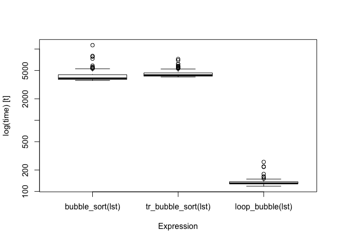
The module primarily solves the problem of exceeding the stack space. The transformed functions are not as fast as those we can code by hand using loops. It should be possible to improve on the running time of the transformed functions, however, with some program analysis… This analysis should be included in the time usage analysis, though, which will probably still come out saying that manually programmed looping versions are faster than transformed functions. Recursive functions can be a lot easier to read, though, than their corresponding looping versions, especially with pattern matching.