The goal of survParamSim is to perform survival simulation with parametric survival model generated from ‘survreg’ function in ‘survival’ package. In each simulation, coefficients are resampled from variance-covariance matrix of parameter estimates, in order to capture uncertainty in model parameters.
You can install the package from CRAN.
This GitHub pages contains function references and vignette. The example below is a sneak peek of example outputs.
First, run survreg to fit parametric survival model:
library(dplyr)
#>
#> Attaching package: 'dplyr'
#> The following objects are masked from 'package:stats':
#>
#>     filter, lag
#> The following objects are masked from 'package:base':
#>
#>     intersect, setdiff, setequal, union
library(ggplot2)
library(survival)
library(survParamSim)

set.seed(12345)

# ref for dataset https://vincentarelbundock.github.io/Rdatasets/doc/survival/colon.html
colon2 <-
  as_tibble(colon) %>%
  # recurrence only and not including Lev alone arm
  filter(rx != "Lev",
         etype == 1) %>%
  # Same definition as Lin et al, 1994
  mutate(rx = factor(rx, levels = c("Obs", "Lev+5FU")),
depth = as.numeric(extent <= 2))Next, run parametric bootstrap simulation:
sim <-
  surv_param_sim(object = fit.colon, newdata = colon2,
                 censor.dur = c(1800, 3000),
                 # Simulating only 100 times to make the example go fast
                 n.rep = 100)

sim
#> ---- Simulated survival data with the following model ----
#> survreg(formula = Surv(time, status) ~ rx + node4 + depth, data = colon2,
#>     dist = "lognormal")
#>
#> * Use `extract_sim()` function to extract individual simulated survivals
#> * Use `calc_km_pi()` function to get survival curves and median survival time
#> * Use `calc_hr_pi()` function to get hazard ratio
#>
#> * Settings:
#>     #simulations: 100
#>     #subjects: 619 (without NA in model variables)
Calculate survival curves with prediction intervals:
km.pi <- calc_km_pi(sim, trt = "rx", group = c("node4", "depth"))

km.pi
#> ---- Simulated and observed (if calculated) survival curves ----
#> * Use `extract_median_surv()` to extract median survival times
#> * Use `extract_km_pi()` to extract prediction intervals of K-M curves
#> * Use `plot_km_pi()` to draw survival curves
#>
#> * Settings:
#>     trt: rx
#>     group: node4
#>     pi.range: 0.95
#>     calc.obs: TRUE
plot_km_pi(km.pi) +
  theme(legend.position = "bottom") +
  labs(y = "Recurrence free rate") +
  expand_limits(y = 0)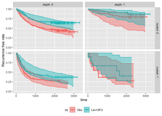
extract_median_surv(km.pi)
#> # A tibble: 32 x 7
#>    rx    node4 depth     n description median quantile
#>    <fct> <dbl> <dbl> <dbl> <chr>        <dbl>    <dbl>
#>  1 Obs       0     0   193 pi_low       1257.    0.025
#>  2 Obs       0     0   193 pi_med       1895.    0.5
#>  3 Obs       0     0   193 pi_high      2713.    0.975
#>  4 Obs       0     0   193 obs          1436    NA
#>  5 Obs       0     1    35 pi_low       1539.    0.025
#>  6 Obs       0     1    35 pi_med       2558.    0.5
#>  7 Obs       0     1    35 pi_high      2913.    0.975
#>  8 Obs       0     1    35 obs            NA    NA
#>  9 Obs       1     0    76 pi_low        264.    0.025
#> 10 Obs       1     0    76 pi_med        451.    0.5
#> # … with 22 more rows
Calculate hazard ratios with prediction intervals:
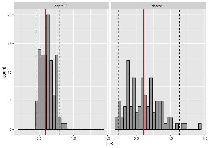
hr.pi <- calc_hr_pi(sim, trt = "rx", group = c("depth"))

hr.pi
#> ---- Simulated and observed (if calculated) hazard ratio ----
#> * Use `extract_hr_pi()` to extract prediction intervals and observed HR
#> * Use `extract_hr()` to extract individual simulated HRs
#> * Use `plot_hr_pi()` to draw histogram of predicted HR
#>
#> * Settings:
#>     trt: rx
#>          (Lev+5FU as test trt, Obs as control)
#>     group: depth
#>     pi.range: 0.95
#>     calc.obs: TRUE
plot_hr_pi(hr.pi)