The goal of supernova is to create ANOVA tables in the format used by Judd, McClelland, and Ryan (2017, ISBN: 978-1138819832) in their introductory textbook, Data Analysis: A Model Comparison Approach to Regression, ANOVA, and Beyond (book website).* These tables include proportional reduction in error, a useful measure for teaching the underlying concepts of ANOVA and regression, and formatting to ease the transition between the book and R.
* Note: we are NOT affiliated with the authors or their institution.
In keeping with the approach in Judd, McClelland, and Ryan (2017), the ANOVA tables in this package are calculated using a model comparison approach that should be understandable given a beginner’s understanding of base R and the information from the book (so if you have these and don’t understand what is going on in the code, let us know because we are missing the mark!). Here is an explanation of how the tables are calculated:
The “Total” row is calculated by updating the model passed to an empty model. For example, lm(mpg ~ hp * disp, data = mtcars) is updated to (lm(mpg ~ NULL, data = mtcars)). From this empty model, the sum of squares and df can be calculated.
If there is at least one predictor in the model, the overall model row and the error row are calculated. In the vernacular of the book, the compact model is represented by the updated empty model from 1 above, and the augmented model is the original model passed to supernova(). From these models the SSE(A) is calculated by sum(resid(null_model) ^ 2), the SSR is calculated by SSE(C) - SSE(A), the PRE for the overall model is extracted from the fit (r.squared), the df for the error row is extracted from the lm() fit (df.residuals).
If there are more than one predictors, the single term deletions are computed using drop1(). For the model y ~ a * b (which expands to y ~ a + b + a:b, where a:b is the interaction of a and b), drop1() essentially creates three models each with one term removed: y ~ a + a:b, y ~ b + a:b, and y ~ a + b. These models are considered the compact models which do not include the tested terms a, b, and a:b, respectively. drop1() computes the SSR (Sum Sq) and SSE(C) (RSS) for each of these augmented and compact model pairs, and these values are used to compute the SSR and PRE for each.
Finally, the MS (SS / df), F (MSR / MSE), and p columns are calculated from already-computed values in the table.
In addition to the ANOVA table provided by supernova(), the supernova package provides some useful functions for extracting estimates from a linear model: b0(), b1(), fVal(), PRE(). These are especially useful in the context of creating bootstrapped sampling distributions as in the Examples below.
The following models are explicitly tested and supported by supernova(), for independent samples (between-subjects) data only. For these models, there is also support for datasets with missing or unbalanced data.
y ~ NULLy ~ ay ~ a + by ~ a * bAnything not included above is not (yet) explicitly tested and may yield errors or incorrect statistics. This includes, but is not limited to
You can install the released version of supernova from CRAN with:
Alternatively you can download the package directly from this repository using devtools:
Here are some basic examples of the code and output for this package:
supernova(lm(mpg ~ NULL, data = mtcars))
#>  Analysis of Variance Table (Type III SS)
#>  Model: mpg ~ NULL
#>
#>                                SS  df     MS   F PRE   p
#>  ----- ----------------- -------- --- ------ --- --- ---
#>  Model (error reduced) |      --- ---    --- --- --- ---
#>  Error (from model)    |      --- ---    --- --- --- ---
#>  ----- ----------------- -------- --- ------ --- --- ---
#> Total (empty model) | 1126.047 31 36.324supernova(lm(mpg ~ hp, data = mtcars))
#> Analysis of Variance Table (Type III SS)
#> Model: mpg ~ hp
#>
#> SS df MS F PRE p
#> ----- ----------------- -------- -- ------- ------ ------ -----
#> Model (error reduced) | 678.373 1 678.373 45.460 0.6024 .0000
#> Error (from model) | 447.674 30 14.922
#> ----- ----------------- -------- -- ------- ------ ------ -----
#> Total (empty model) | 1126.047 31 36.324supernova(lm(mpg ~ hp + disp, data = mtcars))
#> Analysis of Variance Table (Type III SS)
#> Model: mpg ~ hp + disp
#>
#> SS df MS F PRE p
#> ----- ----------------- -------- -- ------- ------ ------ -----
#> Model (error reduced) | 842.554 2 421.277 43.095 0.7482 .0000
#> hp | 33.665 1 33.665 3.444 0.1061 .0737
#> disp | 164.181 1 164.181 16.795 0.3667 .0003
#> Error (from model) | 283.493 29 9.776
#> ----- ----------------- -------- -- ------- ------ ------ -----
#> Total (empty model) | 1126.047 31 36.324supernova(lm(mpg ~ hp * disp, data = mtcars))
#> Analysis of Variance Table (Type III SS)
#> Model: mpg ~ hp * disp
#>
#> SS df MS F PRE p
#> ------- ----------------- -------- -- ------- ------ ------ -----
#> Model (error reduced) | 923.189 3 307.730 42.475 0.8198 .0000
#> hp | 113.393 1 113.393 15.651 0.3586 .0005
#> disp | 188.449 1 188.449 26.011 0.4816 .0000
#> hp:disp | 80.635 1 80.635 11.130 0.2844 .0024
#> Error (from model) | 202.858 28 7.245
#> ------- ----------------- -------- -- ------- ------ ------ -----
#> Total (empty model) | 1126.047 31 36.324These are equivalent to the above:
supernova(lm(mpg ~ hp * disp, data = mtcars), type = 3)
supernova(lm(mpg ~ hp * disp, data = mtcars), type = "III")
supernova(lm(mpg ~ hp * disp, data = mtcars), type = "orthogonal")supernova(lm(mpg ~ hp * disp, data = mtcars), type = 1)
#> Analysis of Variance Table (Type I SS)
#> Model: mpg ~ hp * disp
#>
#> SS df MS F PRE p
#> ------- ----------------- -------- -- ------- ------ ------ -----
#> Model (error reduced) | 923.189 3 307.730 42.475 0.8198 .0000
#> hp | 678.373 1 678.373 93.634 0.7698 .0000
#> disp | 164.181 1 164.181 22.661 0.4473 .0001
#> hp:disp | 80.635 1 80.635 11.130 0.2844 .0024
#> Error (from model) | 202.858 28 7.245
#> ------- ----------------- -------- -- ------- ------ ------ -----
#> Total (empty model) | 1126.047 31 36.324These are equivalent to the above:
supernova(lm(mpg ~ hp * disp, data = mtcars), type = "I")
supernova(lm(mpg ~ hp * disp, data = mtcars), type = "sequential")supernova(lm(mpg ~ hp * disp, data = mtcars), type = 2)
#> Analysis of Variance Table (Type II SS)
#> Model: mpg ~ hp * disp
#>
#> SS df MS F PRE p
#> ------- ----------------- -------- -- ------- ------ ------ -----
#> Model (error reduced) | 923.189 3 307.730 42.475 0.8198 .0000
#> hp | 33.665 1 33.665 4.647 0.1423 .0399
#> disp | 164.181 1 164.181 22.661 0.4473 .0001
#> hp:disp | 80.635 1 80.635 11.130 0.2844 .0024
#> Error (from model) | 202.858 28 7.245
#> ------- ----------------- -------- -- ------- ------ ------ -----
#> Total (empty model) | 1126.047 31 36.324These are equivalent to the above:
supernova(lm(mpg ~ hp * disp, data = mtcars), type = "II")
supernova(lm(mpg ~ hp * disp, data = mtcars), type = "hierarchical")This package is based on a model comparison approach to understanding regression and ANOVA. As such it is useful to know which models are being compared for any given term in an ANOVA table. The generate_models() function accepts a linear model and the desired type of SS and returns a list of the models that should be compared to appropriately evaluate each term in the full model.
generate_models(lm(mpg ~ hp * disp, data = mtcars), type = 2)
#> Comparison Models for Type II SS
#> Model: mpg ~ hp * disp
#>
#> Full Model
#>   complex: mpg ~ hp + disp + hp:disp
#>    simple: mpg ~ NULL
#> hp
#>   complex: mpg ~ hp + disp
#>    simple: mpg ~      disp
#> disp
#>   complex: mpg ~ hp + disp
#>    simple: mpg ~ hp
#> hp:disp
#>   complex: mpg ~ hp + disp + hp:disp
#> simple: mpg ~ hp + dispThe estimate extraction functions in the package simplify the ability to create bootstrapped sampling distributions of those estimates. The functions currently exported are PRE, b0, b1, fVal, SSM/SSR, and SSE. Other terms can be bootstrapped as well, the target estimated just needs to be extracted via other means.
# to extract a single estimate:
b1(lm(mpg ~ hp, data = mtcars))
#> [1] -0.06823

# use mosaic package to repetetively resample to bootstrap a distribution
sd_of_b1 <- mosaic::do(1000) * b1(lm(mpg ~ hp, data = mosaic::resample(mtcars)))

# plot the bootstrapped estimates
hist(sd_of_b1$b1)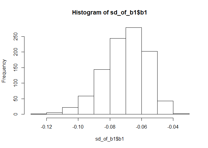
sd_of_hp <- mosaic::do(1000) * {
  # create a new model from the resampled data
  model <- lm(mpg ~ disp * hp, data = mosaic::resample(mtcars))

  # extract the desired estimate, here the coefficient for hp
  coef(model)[["hp"]]
}

# plot the bootstrapped estimates
hist(sd_of_hp$result)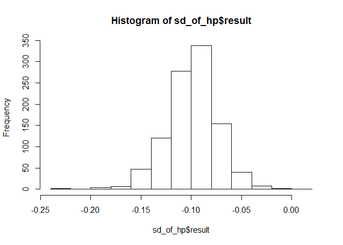
If you see an issue, problem, or improvement that you think we should know about, or you think would fit with this package, please let us know on our issues page. Alternatively, if you are up for a little coding of your own, submit a pull request:
git checkout -b my-new-featuregit commit -am 'Add some feature'git push origin my-new-feature