


statsExpressions: Expressions with statistical details| Package | Status | Usage | GitHub | References |
|---|---|---|---|---|
|
||||
|
|
|||
|
||||
|
|
statsExpressions provides statistical processing backend for the ggstatsplot package, which combines ggplot2 visualizations with expressions containing results from statistical tests. statsExpressions contains all functions needed to create these expressions.
To get the latest, stable CRAN release:
You can get the development version of the package from GitHub. To see what new changes (and bug fixes) have been made to the package since the last release on CRAN, you can check the detailed log of changes here: https://indrajeetpatil.github.io/statsExpressions/news/index.html
If you are in hurry and want to reduce the time of installation, prefer-
# needed package to download from GitHub repo
install.packages("remotes")

# downloading the package from GitHub
remotes::install_github(
  repo = "IndrajeetPatil/statsExpressions", # package path on GitHub
  dependencies = FALSE, # assumes you have already installed needed packages
  quick = TRUE # skips docs, demos, and vignettes
)
If time is not a constraint-
remotes::install_github(
  repo = "IndrajeetPatil/statsExpressions", # package path on GitHub
  dependencies = TRUE, # installs packages which statsExpressions depends on
  upgrade_dependencies = TRUE # updates any out of date dependencies
)If you want to cite this package in a scientific journal or in any other context, run the following code in your R console:
To see the documentation relevant for the development version of the package, see the dedicated website for statsExpressions, which is updated after every new commit: https://indrajeetpatil.github.io/statsExpressions/.
Currently, it supports only the most common types of statistical tests. Specifically, parametric, non-parametric, robust, and bayesian versions of:
The table below summarizes all the different types of analyses currently supported in this package-
| Description | Parametric | Non-parametric | Robust | Bayes Factor |
|---|---|---|---|---|
| Between group/condition comparisons | Yes | Yes | Yes | Yes |
| Within group/condition comparisons | Yes | Yes | Yes | Yes |
| Distribution of a numeric variable | Yes | Yes | Yes | Yes |
| Correlation between two variables | Yes | Yes | Yes | Yes |
| Association between categorical variables | Yes | NA |
NA |
Yes |
| Equal proportions for categorical variable levels | Yes | NA |
NA |
Yes |
| Random-effects meta-analysis | Yes | No | Yes | Yes |
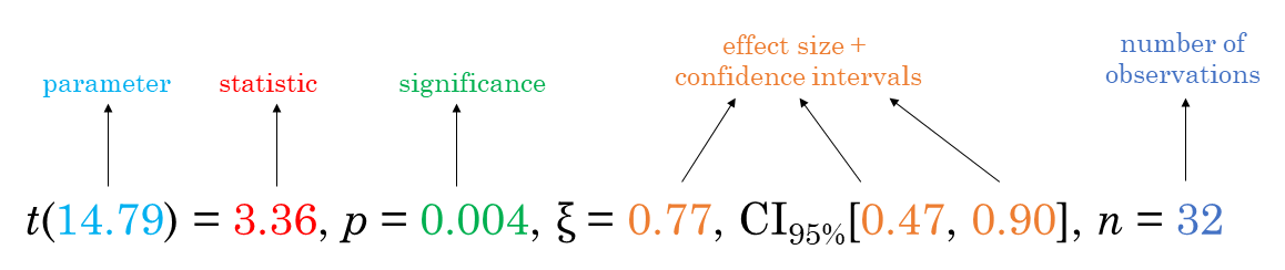
For all statistical test expressions, the default template abides by the APA gold standard for statistical reporting. For example, here are results from Yuen’s test for trimmed means (robust t-test):
Here is a summary table of all the statistical tests currently supported across various functions: https://indrajeetpatil.github.io/statsExpressions/articles/stats_details.html
A list of primary functions in this package can be found at the package website: https://indrajeetpatil.github.io/statsExpressions/reference/index.html
Following are few examples of how these functions can be used.
Let’s say we want to check differences in weight of the vehicle based on number of cylinders in the engine and wish to carry out Welch’s ANOVA:
# setup
set.seed(123)
library(ggplot2)
library(statsExpressions)
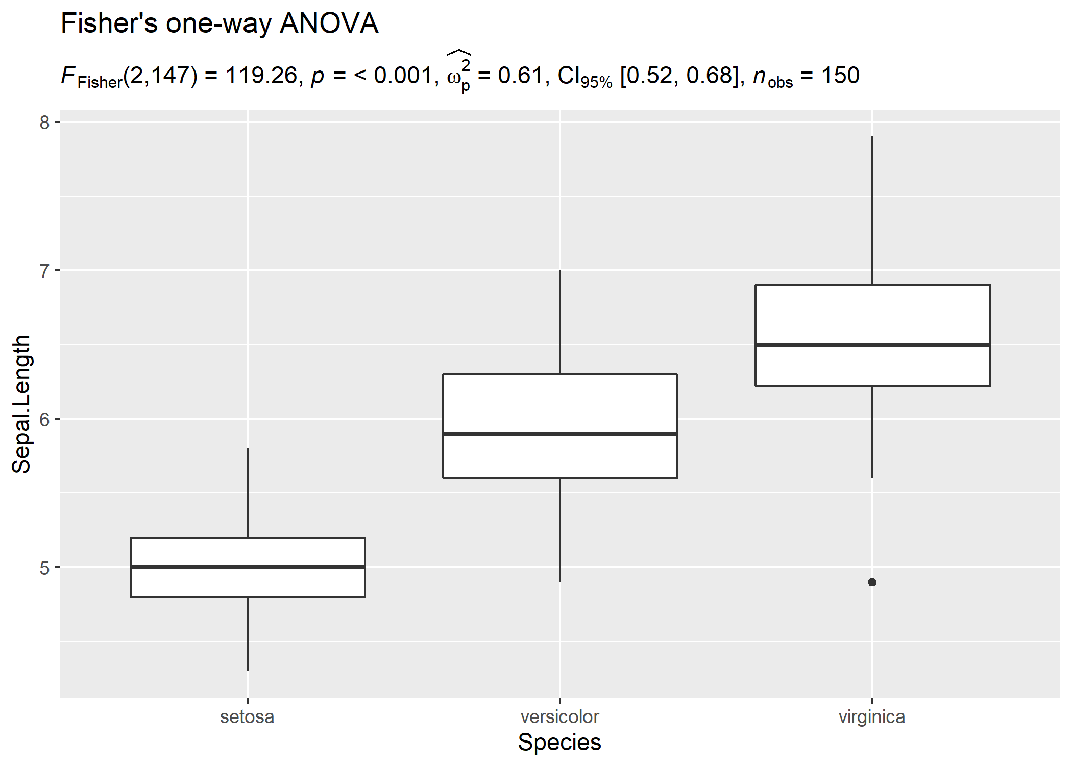
# create a boxplot
ggplot(iris, aes(x = Species, y = Sepal.Length)) +
geom_boxplot() +
labs(
title = "Fisher's one-way ANOVA",
subtitle = expr_anova_parametric(iris, Species, Sepal.Length, var.equal = TRUE)
)
In case you change your mind and now want to carry out a robust ANOVA instead. Also, let’s use a different kind of a visualization:
# setup
set.seed(123)
library(ggplot2)
library(statsExpressions)
library(ggridges)

# create a ridgeplot
ggplot(iris, aes(x = Sepal.Length, y = Species)) +
  geom_density_ridges(
    jittered_points = TRUE, quantile_lines = TRUE,
    scale = 0.9, vline_size = 1, vline_color = "red",
    position = position_raincloud(adjust_vlines = TRUE)
  ) +
  labs(
    title = "A heteroscedastic one-way ANOVA for trimmed means",
    subtitle = expr_anova_robust(iris, Species, Sepal.Length)
  )
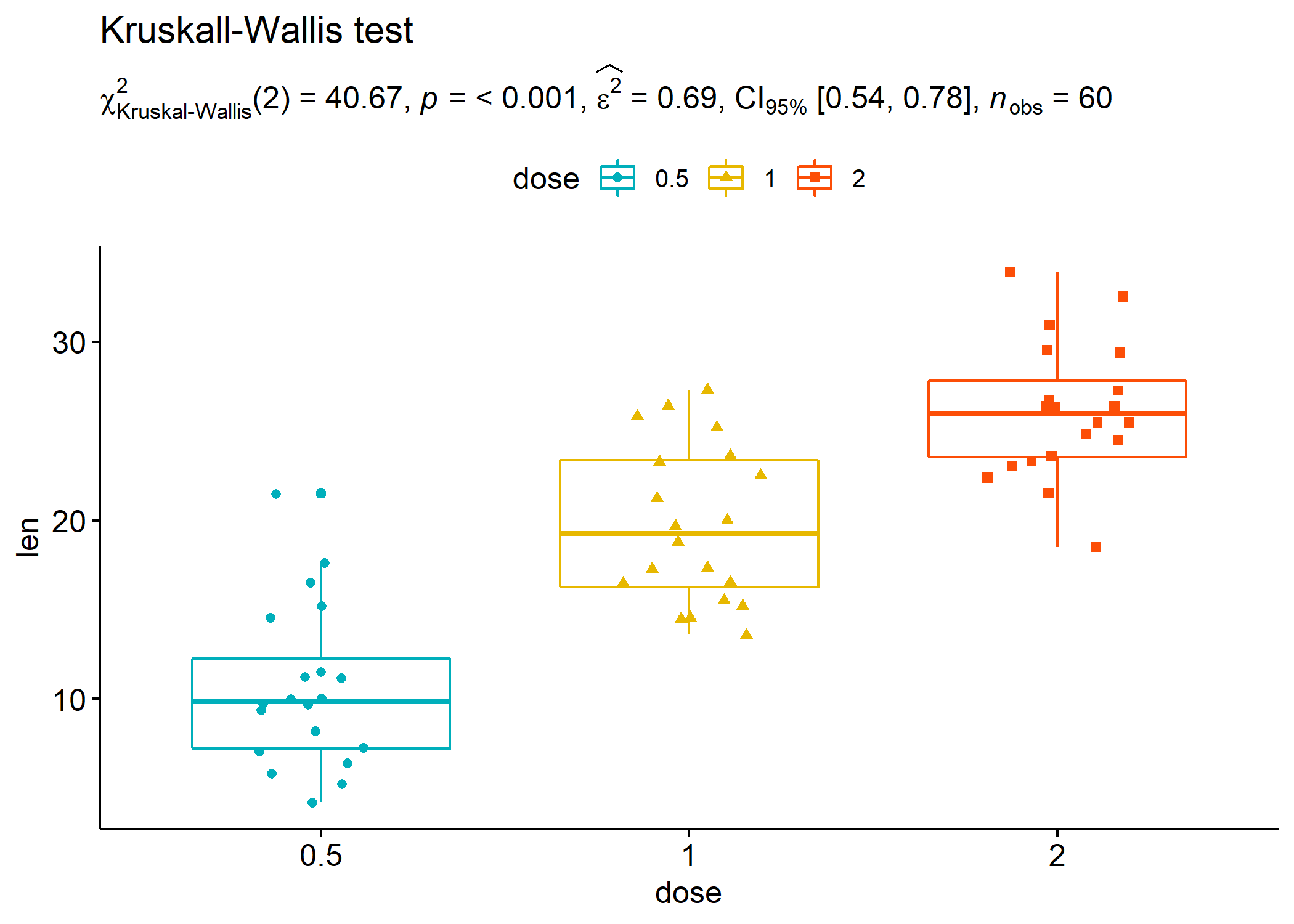
Needless to say, you can also use these functions to display results in ggplot-extension packages. For example, ggpubr:
set.seed(123)
library(ggpubr)
library(ggplot2)

# plot
ggboxplot(
  ToothGrowth,
  x = "dose",
  y = "len",
  color = "dose",
  palette = c("#00AFBB", "#E7B800", "#FC4E07"),
  add = "jitter",
  shape = "dose"
) + # adding results from stats analysis using `statsExpressions`
  labs(
    title = "Kruskall-Wallis test",
    subtitle = expr_anova_nonparametric(ToothGrowth, dose, len, type = "np")
  )
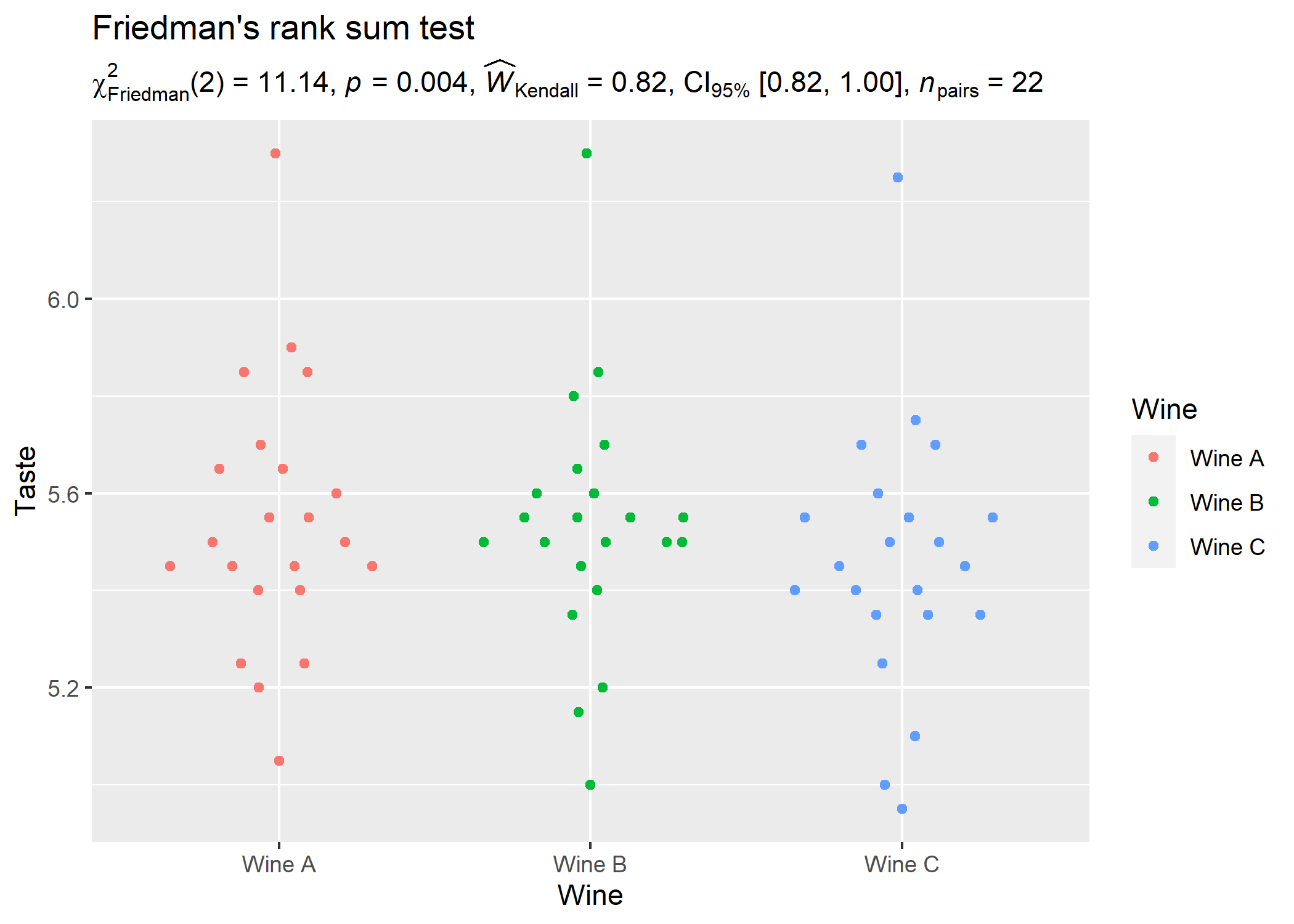
Let’s now see an example of a repeated measures one-way ANOVA.
# setup
set.seed(123)
library(ggplot2)
library(WRS2)
library(ggbeeswarm)
library(statsExpressions)

ggplot2::ggplot(WineTasting, aes(Wine, Taste, color = Wine)) +
  geom_quasirandom() +
  labs(
    title = "Friedman's rank sum test",
    subtitle = expr_anova_nonparametric(WineTasting, Wine, Taste, paired = TRUE, type = "np")
  )
# setup
set.seed(123)
library(ggplot2)
library(hrbrthemes)
library(statsExpressions)
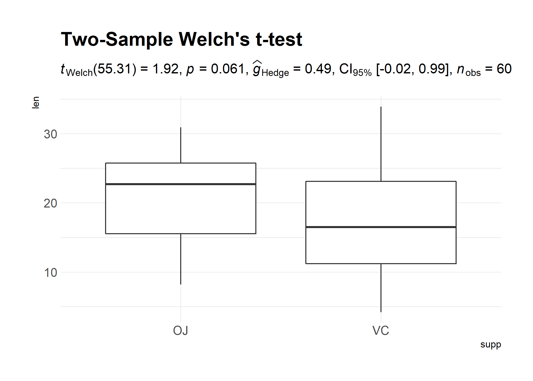
# create a plot
ggplot(ToothGrowth, aes(supp, len)) +
geom_boxplot() +
theme_ipsum_rc() +
# adding a subtitle with
labs(
title = "Two-Sample Welch's t-test",
subtitle = expr_t_parametric(ToothGrowth, supp, len)
)
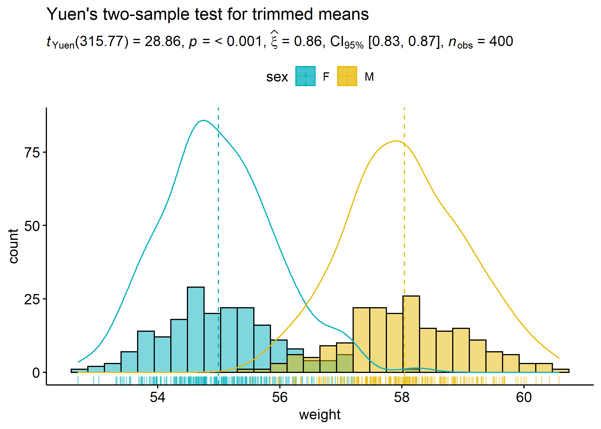
Example with ggpubr:
# setup
set.seed(123)
library(ggplot2)
library(ggpubr)
library(statsExpressions)

# basic plot
gghistogram(
  data.frame(
    sex = factor(rep(c("F", "M"), each = 200)),
    weight = c(rnorm(200, 55), rnorm(200, 58))
  ),
  x = "weight",
  add = "mean",
  rug = TRUE,
  fill = "sex",
  palette = c("#00AFBB", "#E7B800"),
  add_density = TRUE
) + # displaying stats results
  labs(
    title = "Yuen's two-sample test for trimmed means",
    subtitle = expr_t_robust(
      data = data.frame(
        sex = factor(rep(c("F", "M"), each = 200)),
        weight = c(rnorm(200, 55), rnorm(200, 58))
      ),
      x = sex,
      y = weight,
      type = "robust",
      messages = FALSE
    )
  )
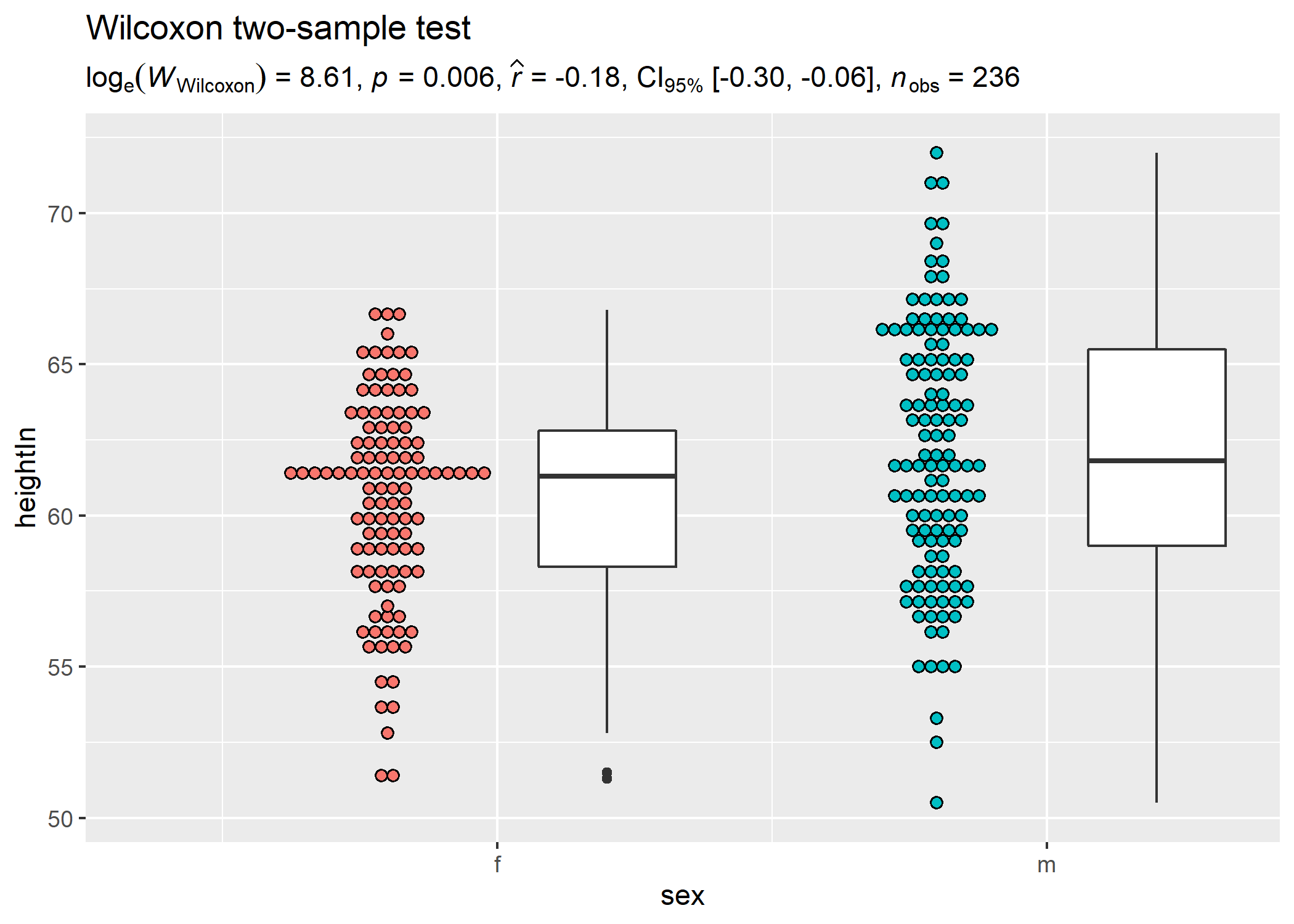
Another example with ggiraphExtra:
# setup
set.seed(123)
library(ggplot2)
library(ggiraphExtra)
library(gcookbook)
library(statsExpressions)

# plot
ggDot(heightweight, aes(sex, heightIn, fill = sex),
  boxfill = "white",
  binwidth = 0.4
) +
  labs(
    title = "Wilcoxon two-sample test",
    subtitle = expr_t_nonparametric(heightweight, sex, heightIn, type = "np")
  )
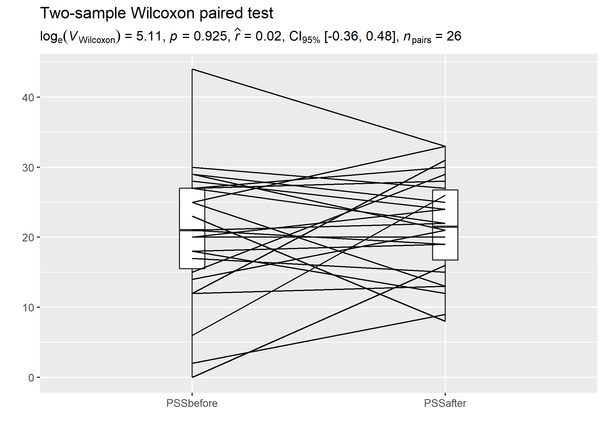
We can also have a look at a repeated measures design and the related expressions.
# setup
set.seed(123)
library(ggplot2)
library(statsExpressions)
library(tidyr)
library(PairedData)
data(PrisonStress)

# plot
paired.plotProfiles(PrisonStress, "PSSbefore", "PSSafter", subjects = "Subject") +
  # `statsExpressions` needs data in the tidy format
  labs(
    title = "Two-sample Wilcoxon paired test",
    subtitle = expr_t_nonparametric(
      data = pivot_longer(PrisonStress, starts_with("PSS"), "PSS", values_to = "stress"),
      x = PSS,
      y = stress,
      paired = TRUE
    )
  )
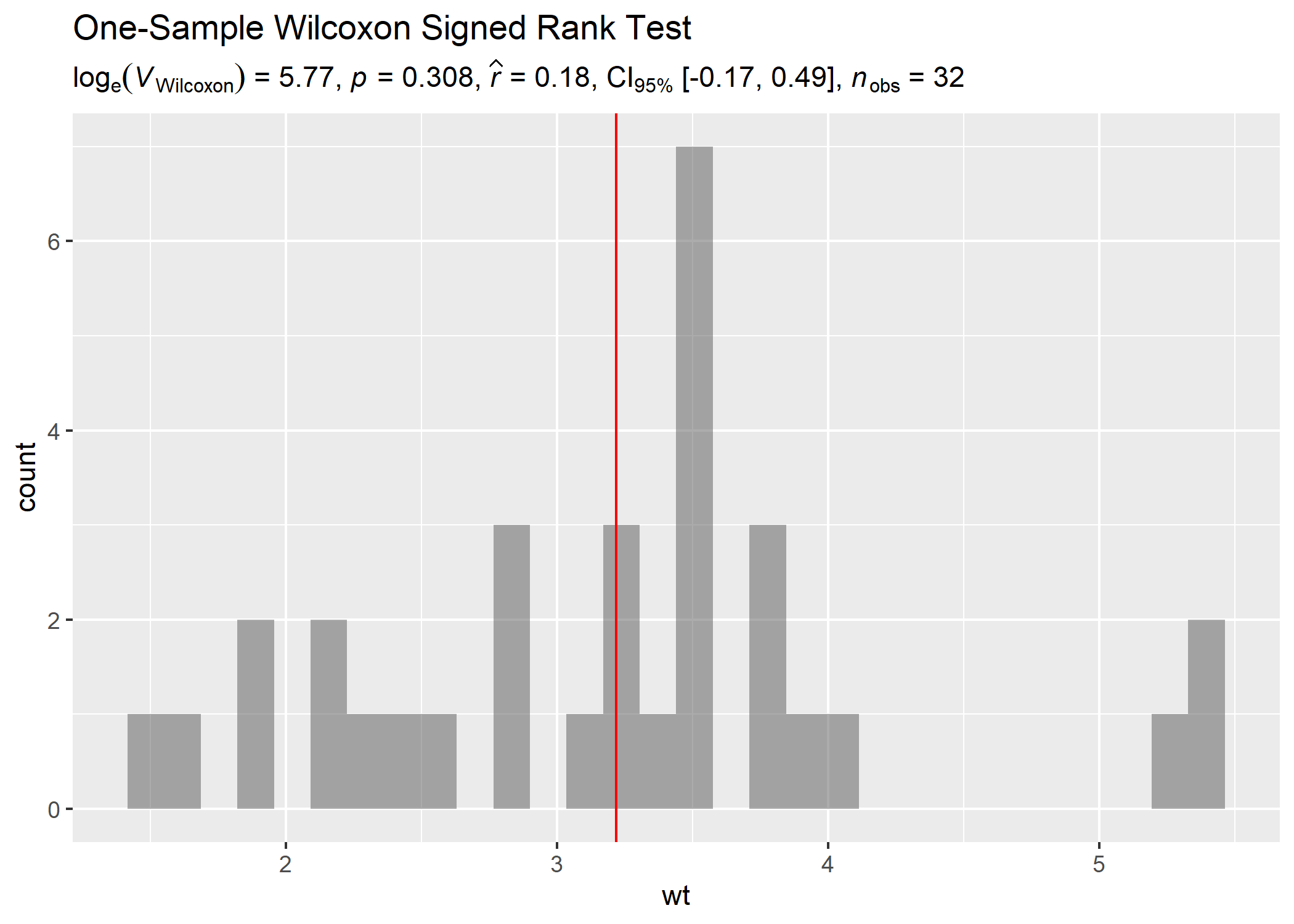
# setup
set.seed(123)
library(ggplot2)
library(statsExpressions)

# creating a histogram plot
ggplot(mtcars, aes(wt)) +
  geom_histogram(alpha = 0.5) +
  geom_vline(xintercept = mean(mtcars$wt), color = "red") +
  # adding a caption with a non-parametric one-sample test
  labs(
    title = "One-Sample Wilcoxon Signed Rank Test",
    subtitle = expr_t_onesample(mtcars, wt, test.value = 3, type = "nonparametric")
  )
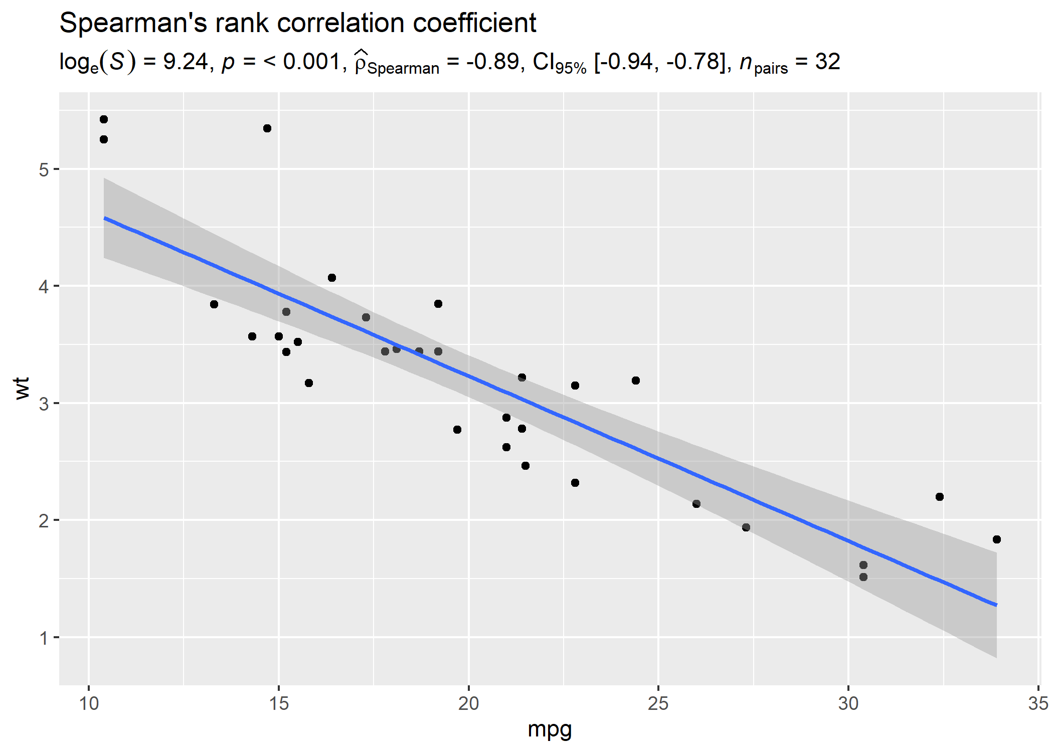
Let’s look at another example where we want to run correlation analysis:
# setup
set.seed(123)
library(ggplot2)
library(statsExpressions)

# create a ridgeplot
ggplot(mtcars, aes(mpg, wt)) +
  geom_point() +
  geom_smooth(method = "lm") +
  labs(
    title = "Spearman's rank correlation coefficient",
    subtitle = expr_corr_test(mtcars, mpg, wt, type = "nonparametric")
  )
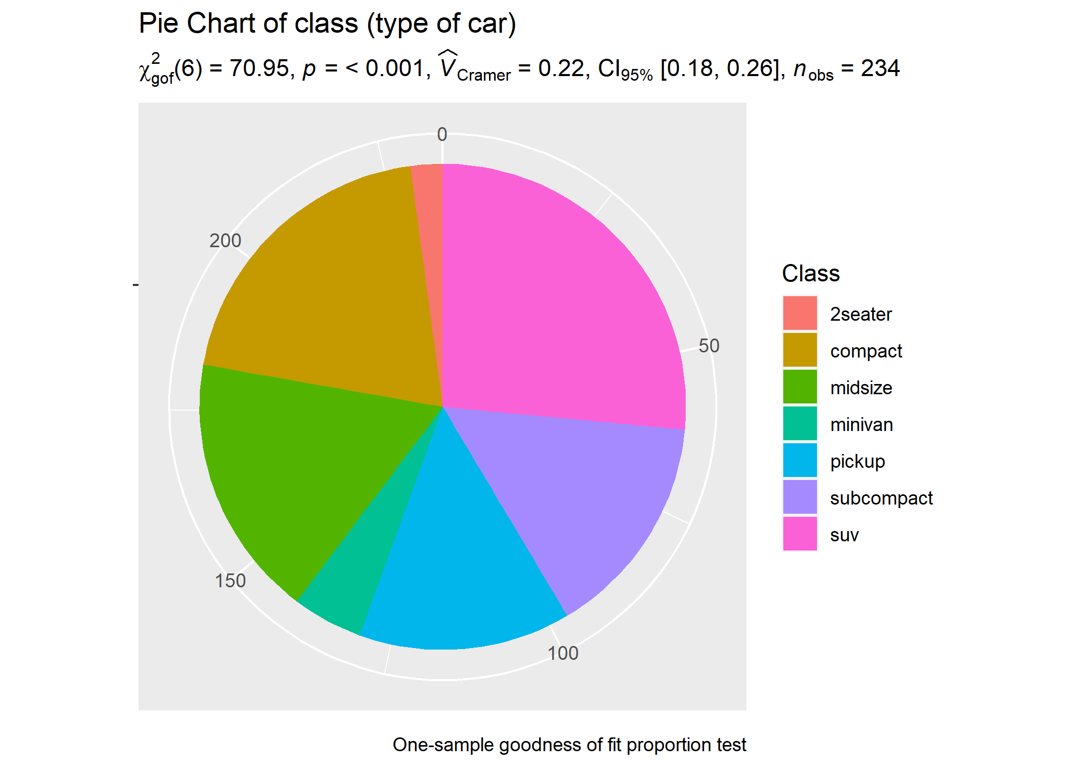
For categorical/nominal data
# setup
set.seed(123)
library(ggplot2)
library(statsExpressions)

# basic pie chart
ggplot(as.data.frame(table(mpg$class)), aes(x = "", y = Freq, fill = factor(Var1))) +
  geom_bar(width = 1, stat = "identity") +
  theme(axis.line = element_blank()) +
  # cleaning up the chart and adding results from one-sample proportion test
  coord_polar(theta = "y", start = 0) +
  labs(
    fill = "Class",
    x = NULL,
    y = NULL,
    title = "Pie Chart of class (type of car)",
    subtitle = expr_onesample_proptest(as.data.frame(table(mpg$class)), Var1, counts = Freq),
    caption = "One-sample goodness of fit proportion test"
  )
You can also use these function to get the expression in return without having to display them in plots:
# setup
set.seed(123)
library(ggplot2)
library(statsExpressions)

# Pearson's chi-squared test of independence
expr_contingency_tab(mtcars, am, cyl)
#> paste(NULL, chi["Pearson"]^2, "(", "2", ") = ", "8.74", ", ",
#>     italic("p"), " = ", "0.013", ", ", widehat(italic("V"))["Cramer"],
#>     " = ", "0.46", ", CI"["95%"], " [", "0.08", ", ", "0.75",
#> "]", ", ", italic("n")["obs"], " = ", 32L)# setup
set.seed(123)
library(metaviz)
library(ggplot2)
# meta-analysis forest plot with results random-effects meta-analysis
viz_forest(
x = mozart[, c("d", "se")],
study_labels = mozart[, "study_name"],
xlab = "Cohen's d",
variant = "thick",
type = "cumulative"
) + # use `statsExpressions` to create expression containing results
labs(
title = "Meta-analysis of Pietschnig, Voracek, and Formann (2010) on the Mozart effect",
subtitle = expr_meta_parametric(dplyr::rename(mozart, estimate = d, std.error = se))
) +
theme(text = element_text(size = 12))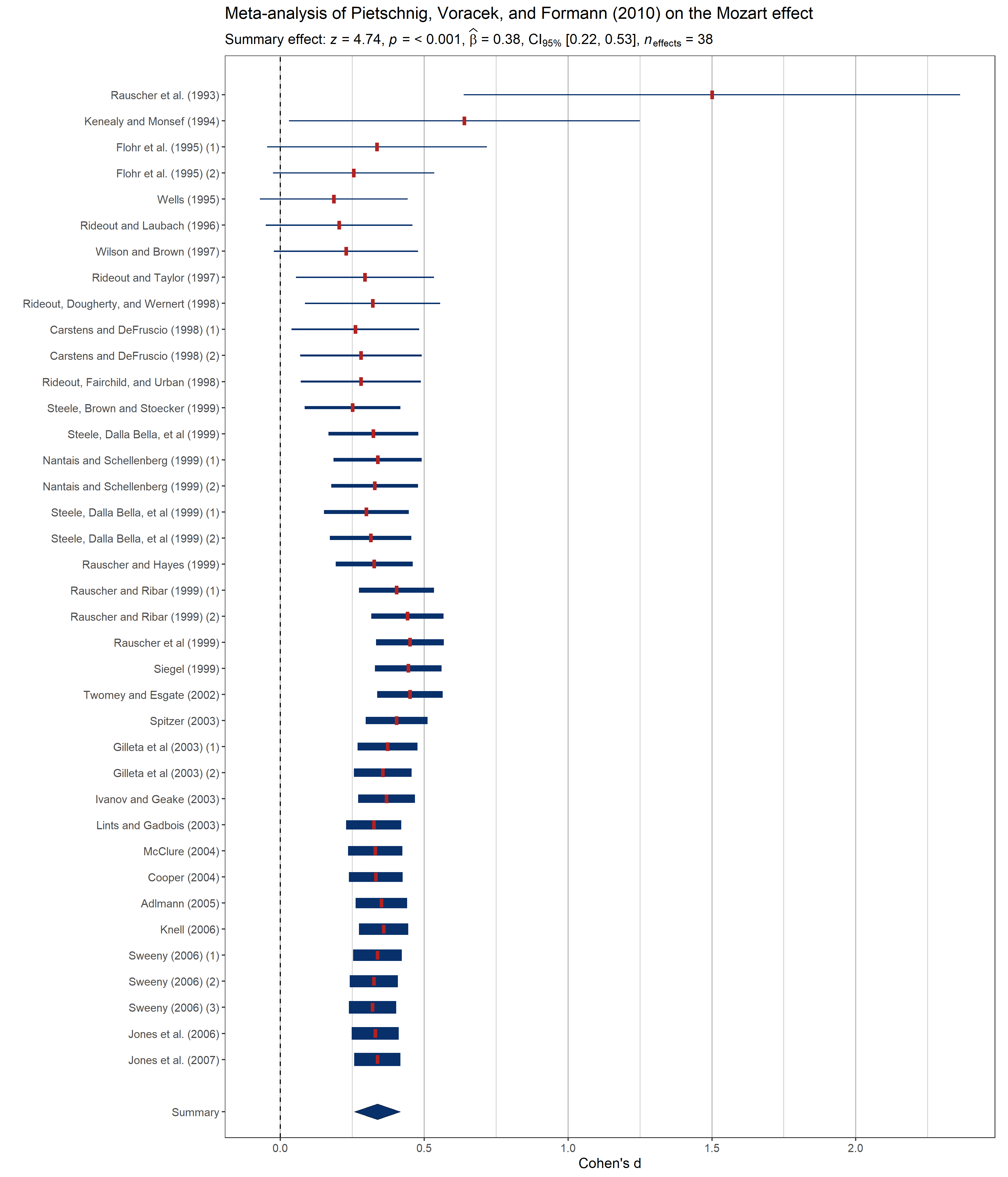
ggstatsplotNote that these functions were initially written to display results from statistical tests on ready-made ggplot2 plots implemented in ggstatsplot.
For detailed documentation, see the package website: https://indrajeetpatil.github.io/ggstatsplot/
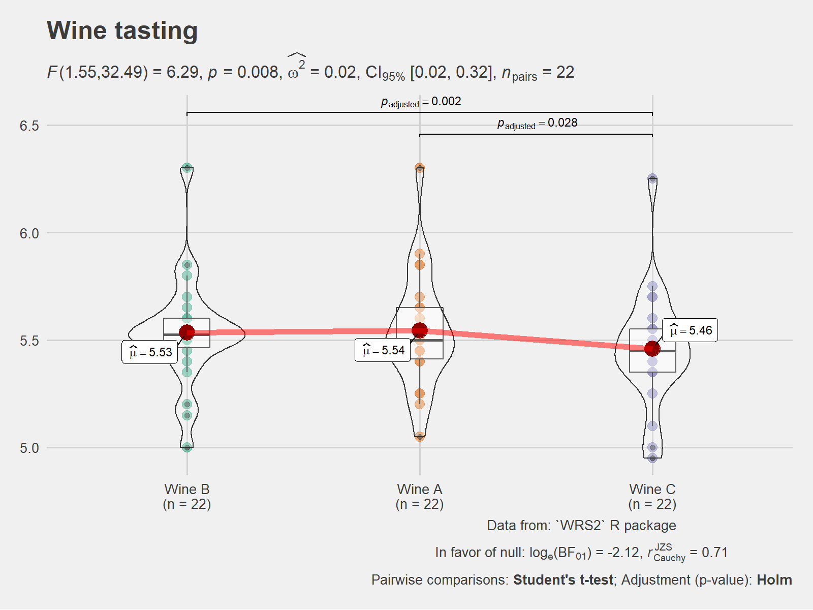
Here is an example from ggstatsplot of what the plots look like when the expressions are displayed in the subtitle-
The hexsticker was generously designed by Sarah Otterstetter (Max Planck Institute for Human Development, Berlin).
As the code stands right now, here is the code coverage for all primary functions involved: https://codecov.io/gh/IndrajeetPatil/statsExpressions/tree/master/R
I’m happy to receive bug reports, suggestions, questions, and (most of all) contributions to fix problems and add features. I personally prefer using the GitHub issues system over trying to reach out to me in other ways (personal e-mail, Twitter, etc.). Pull Requests for contributions are encouraged.
Here are some simple ways in which you can contribute (in the increasing order of commitment):
Read and correct any inconsistencies in the documentation
Raise issues about bugs or wanted features
Review code
Add new functionality (in the form of new plotting functions or helpers for preparing subtitles)
Please note that this project is released with a Contributor Code of Conduct. By participating in this project you agree to abide by its terms.