
![]()
stagedtrees is a package that implements staged event trees, a probability model for discrete random variables.
#stable version from CRAN
install.packages("stagedtrees")

#development version from github
# install.packages("devtools")
devtools::install_github("gherardovarando/stagedtrees")With the stagedtrees package it is possible to fit (stratified) staged event trees to data, use them to compute probabilities, make predictions, visualize and compare different models.
A staged event tree object (sevt class) can be created with the function staged_ev_tree, or with the functions indep and full. In general we create a staged event tree from data in a data.frame or table object.
# Load the PhDArticles data
data("PhDArticles")

# Create the independence model
mod_indep <- indep(PhDArticles, lambda = 1)
mod_indep
#> Staged event tree (fitted)
#> Articles[3] -> Gender[2] -> Kids[2] -> Married[2] -> Mentor[3] -> Prestige[2]
#> 'log Lik.' -4407.498 (df=8)

#Create the full (saturated) model
mod_full <- full(PhDArticles, lambda = 1)
mod_full
#> Staged event tree (fitted)
#> Articles[3] -> Gender[2] -> Kids[2] -> Married[2] -> Mentor[3] -> Prestige[2]
#> 'log Lik.' -4066.97 (df=143)Starting from the independence model of the full model it is
possible to perform automatic model selection.
This methods perform optimization of the model for a given score using different types of heuristic methods.
hc.sevt(object, score, max_iter, trace)mod1 <- hc.sevt(mod_indep)
mod1
#> Staged event tree (fitted)
#> Articles[3] -> Gender[2] -> Kids[2] -> Married[2] -> Mentor[3] -> Prestige[2]
#> 'log Lik.' -4118.434 (df=14)bhc.sevt(object, score, max_iter, trace)mod2 <- bhc.sevt(mod_full)
mod2
#> Staged event tree (fitted)
#> Articles[3] -> Gender[2] -> Kids[2] -> Married[2] -> Mentor[3] -> Prestige[2]
#> 'log Lik.' -4086.254 (df=19)fbhc.sevt(object, score, max_iter, trace)mod3 <- fbhc.sevt(mod_full, score = function(x) -BIC(x))
mod3
#> Staged event tree (fitted)
#> Articles[3] -> Gender[2] -> Kids[2] -> Married[2] -> Mentor[3] -> Prestige[2]
#> 'log Lik.' -4146.642 (df=14)bj.sevt(full, distance, thr, trace, ...)mod4 <- bj.sevt(mod_full)
mod4
#> Staged event tree (fitted)
#> Articles[3] -> Gender[2] -> Kids[2] -> Married[2] -> Mentor[3] -> Prestige[2]
#> 'log Lik.' -4090.79 (df=22)naive.sevt(full, distance, k)mod5 <- naive.sevt(mod_full)
mod5
#> Staged event tree (fitted)
#> Articles[3] -> Gender[2] -> Kids[2] -> Married[2] -> Mentor[3] -> Prestige[2]
#> 'log Lik.' -4118.437 (df=14)%>%The pipe operator from the magrittr package can be used to combine easily various model selection algorithms and to specify models easily.
library(magrittr)
model <- PhDArticles %>% full(lambda = 1) %>% naive.sevt %>%
hc.sevt
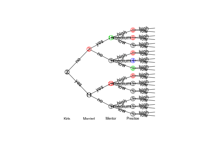
## extract a sub_tree and join two stages
sub_model <- model %>% subtree.sevt(path = c(">2")) %>%
join_stages("Mentor", "1", "2")Obtain marginal probabilities with the prob.sevt function.
# estimated probability of c(Gender = "male", Married = "yes")
# using different models
prob.sevt(mod_indep, c(Gender = "male", Married = "yes"))
#> [1] 0.3573183
prob.sevt(mod3, c(Gender = "male", Married = "yes"))
#> [1] 0.3934668
Or for a data.frame of observations:
obs <- expand.grid(mod_full$tree[c(2,3,5)])
p <- prob.sevt(mod2, obs)
cbind(obs, P = p)
#>    Gender Kids Mentor          P
#> 1    male  yes    low 0.07208877
#> 2  female  yes    low 0.03176117
#> 3    male   no    low 0.09832136
#> 4  female   no    low 0.11463987
#> 5    male  yes medium 0.09915181
#> 6  female  yes medium 0.03452265
#> 7    male   no medium 0.10643086
#> 8  female   no medium 0.14830958
#> 9    male  yes   high 0.08660225
#> 10 female  yes   high 0.02187397
#> 11   male   no   high 0.07702539
#> 12 female no high 0.10927233A staged event tree object can be used to make predictions with the predict method. The class variable can be specified, otherwise the first variable (root) in the tree will be used.
## check accuracy over the PhDArticles data
predicted <- predict(mod3, newdata = PhDArticles)
table(predicted, PhDArticles$Articles)
#>
#> predicted   0 1-2  >2
#>       0    32  34  19
#>       1-2 225 351 149
#>       >2   18  39  48
Conditional probabilities (or log-) can be obtained setting prob = TRUE:
## obtain estimated conditional probabilities in mod3 for first 5 obs
## P(Articles|Gender, Kids, Married, Mentor, Prestige)
predict(mod3, newdata = PhDArticles[1:5,], prob = TRUE)
#>           0       1-2        >2
#> 1 0.2853346 0.4393739 0.2752915
#> 2 0.3186093 0.4906121 0.1907785
#> 3 0.3186093 0.4906121 0.1907785
#> 4 0.3450547 0.5313342 0.1236111
#> 5 0.2304826 0.6315078 0.1380096sample.sevt(mod4, 5)
#> Articles Gender Kids Married Mentor Prestige
#> 1 0 male no no medium low
#> 2 0 female no no low high
#> 3 >2 female no yes high high
#> 4 1-2 male yes yes low high
#> 5 0 male yes yes low high# Degrees of freedom
df.sevt(mod_full)
#> [1] 143
df.sevt(mod_indep)
#> [1] 8
# variables
varnames.sevt(mod1)
#> [1] "Articles" "Gender" "Kids" "Married" "Mentor" "Prestige"
# number of variables
nvar.sevt(mod1)
#> [1] 6plot(mod4, main = "Staged tree learned with bj.sevt",
cex.label.edges = 0.6, cex.nodes = 1.5)
text(mod4, y = -0.03, cex = 0.7)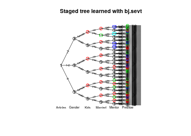
summary(mod4)
#> Call:
#> bj.sevt(mod_full)
#> lambda:  1
#> Stages:
#>   Variable:  Articles
#>  stage npaths sample.size         0      1-2        >2
#>      1      0         915 0.3006536 0.462963 0.2363834
#>   ------------
#>   Variable:  Gender
#>  stage npaths sample.size      male    female
#>      1      3         915 0.5398037 0.4601963
#>   ------------
#>   Variable:  Kids
#>  stage npaths sample.size       yes        no
#>      1      3         494 0.4778226 0.5221774
#>      2      3         421 0.1914894 0.8085106
#>   ------------
#>   Variable:  Married
#>  stage npaths sample.size          no       yes
#>      1      5         303 0.003278689 0.9967213
#>      2      6         599 0.515806988 0.4841930
#>     11      1          13 0.066666667 0.9333333
#>   ------------
#>   Variable:  Mentor
#>  stage npaths sample.size       low    medium       high
#>      1     13         431 0.2557604 0.4377880 0.30645161
#>      2      4         242 0.4367347 0.3346939 0.22857143
#>      3      3         102 0.5142857 0.4000000 0.08571429
#>     18      3         127 0.1307692 0.3384615 0.53076923
#>     22      1          13 0.4375000 0.1875000 0.37500000
#>   ------------
#>   Variable:  Prestige
#>  stage npaths sample.size       low      high
#>      1     36         338 0.5323529 0.4676471
#>      4     14         274 0.6920290 0.3079710
#>      6     15         194 0.3622449 0.6377551
#>      8      7         109 0.1801802 0.8198198
#> ------------A subtree can be extracted, the result is another staged event tree object in the remaining variables.
Check if models are equal.
compare.sevt(mod1, mod2)
#> [1] FALSE

compare.sevt(mod1, mod2, method = "hamming", plot = TRUE,
             cex.label.nodes = 0, cex.label.edges = 0)
#> [1] FALSE
text(mod1)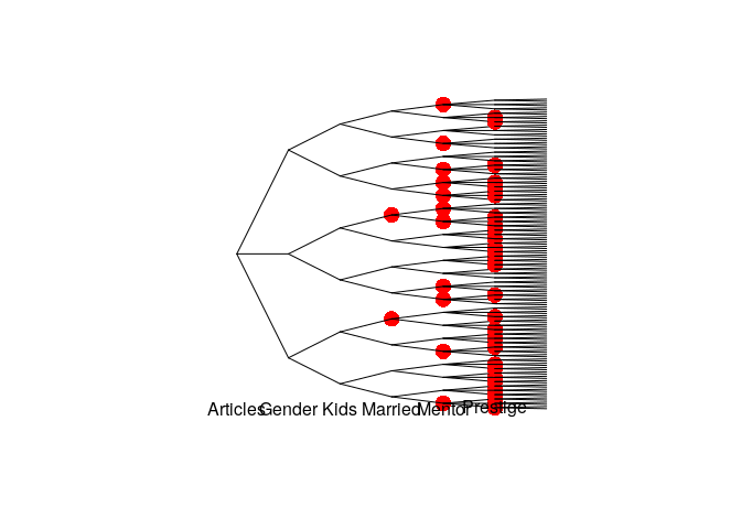
hamming.sevt(mod1, mod2)
#> [1] 43

difftree <- compare.sevt(mod1, mod2, method = "stages", plot = FALSE,
             return.tree = TRUE)

difftree$Married
#>  [1] 0 1 0 1 0 1 0 1 0 1 0 1
Penalized log-likelihood.