library(sparrpowR)
set.seed(1234)
# ----------------- #
# Run spatial_power #
# ----------------- #
# Circular window with radius 0.5
# Uniform case sampling within a disc of radius of 0.1 at the center of the window
# Complete Spatial Randomness control sampling
# 20% prevalence (n = 300 total locations)
# Statistical power to detect both case and control relative clustering
# 100 simulations (more recommended for power calculation)
unit.circle <- spatstat::disc(radius = 0.5, centre = c(0.5,0.5))
foo <- spatial_power(win = unit.circle,
sim_total = 100,
x_case = 0.5,
y_case = 0.5,
samp_case = "uniform",
samp_control = "CSR",
r_case = 0.1,
n_case = 50,
n_control = 250,
cascon = TRUE)
# ----------------------- #
# Outputs from iterations #
# ----------------------- #
# Mean and standard deviation of simulated sample sizes and bandwidth
stats::mean(foo$n_con); stats::sd(foo$n_con) # controls
stats::mean(foo$n_cas); stats::sd(foo$n_cas) # cases
stats::mean(foo$bandw); stats::sd(foo$bandw) # bandwidth of case density (if fixed, same for control density)
# Global Test Statistics
## Global maximum relative risk: Null hypothesis is mu = 1
stats::t.test(x = foo$s_obs, mu = 0, alternative = "two.sided")
## Integral of log relative risk: Null hypothesis is mu = 0
stats::t.test(x = foo$t_obs, mu = 1, alternative = "two.sided")
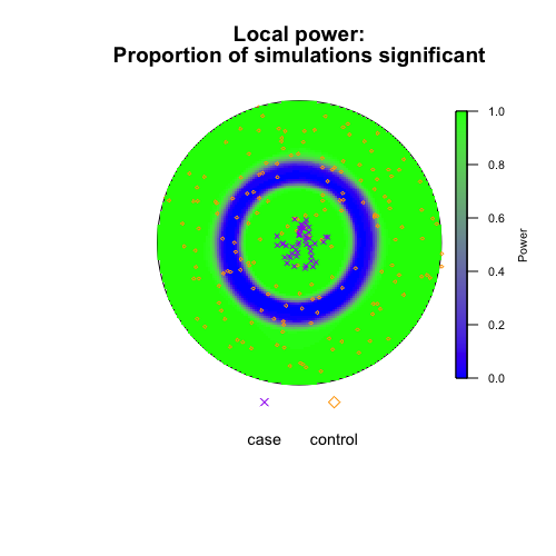
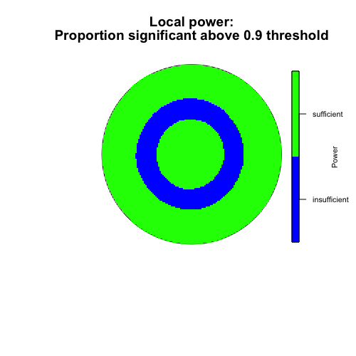
# ----------------- #
# Run spatial_plots #
# ----------------- #
spatial_plots(foo,
p_thresh = 0.9,
chars = c(4,5),
sizes = c(0.6,0.3),
cols = c("blue", "green", "red", "purple", "orange"))