smoots

The goal of smoots is to provide an easy way to estimate the nonparametric trend and its derivatives in equidistant time series with short-memory stationary errors. The main functions allow for data-driven estimates via local polynomial regression with an automatically selected optimal bandwidth.

Installation

You can install the released version of smoots from CRAN with:

install.packages("smoots")

Example

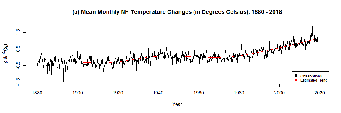
This is a basic example which shows you how to solve a common problem. The data tempNH in the package includes the mean monthly temperature changes in degrees Celsius of the Northern Hemisphere (NH) from 1880 to 2018. The data was obtained from the Goddard Institute for Space Studies of the National Aeronautics and Space Administration (NASA). Let (n) be the number of observations. The data is assumed to follow an additive model

[y_{t} = m(x_{t}) + _{t},]

where (t=1, , n), (y_{t}) are the observed values, (x_{t} = t/n) are the rescaled observation time points on the closed interval between (0) and (1), (m(x_{t})) is a smooth trend function and ({t}) is a zero-mean stationary error term. The user-friendly and simply applicable function msmooth() for the estimation of (m(x{t})) in the additive model will be used.

library(smoots)          # Call the package

data <- tempNH           # Call the 'tempNH' data frame
Yt <- data$Change        # Store the actual values as a vector 

# Estimate the trend function via the 'smoots' package
results <- msmooth(Yt, p = 1, mu = 1, bStart = 0.15, alg = "A")

# Easily access the main estimation results
b.opt <- results$b0             # The optimal bandwidth
trend <- results$ye             # The trend estimates  
resid <- results$res            # The residuals
b.opt
#> [1] 0.101089

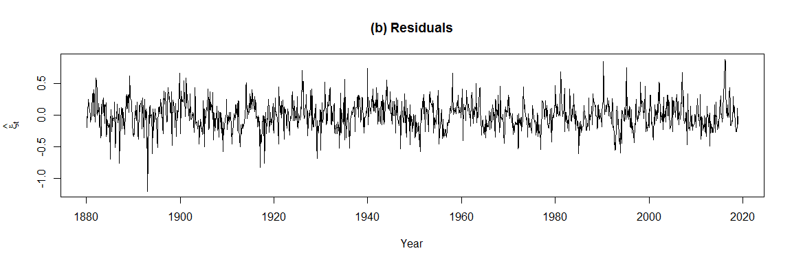
An optimal bandwidth of (0.1009) was selected by the iterative plug-in algorithm (IPI) within msmooth(). Moreover, the estimated trend fits the data suitably and the residuals seem to be stationary. Since the trend was obtained without any parametric assumpions with respect to (_{t}), the residuals could now be further analyzed by means of any suitable parametric approach, e.g. autoregressive-moving-average (ARMA) models.

Further applications

The functions can also be used for the implementation of semiparametric generalized autoregressive conditional heteroskedasticity (Semi-GARCH) models and its various variants in Financial Econometrics (see also the examples in the documentation of msmooth() and tsmooth()).

Functions

In smoots five functions are available.

• dsmooth: Data-driven Local Polynomial for the Trend’s Derivatives in Equidistant Time Series
• gsmooth: Estimation of Trends and their Derivatives via Local Polynomial Regression
• knsmooth: Estimation of Nonparametric Trend Functions via Kernel Regression
• msmooth: Data-driven Nonparametric Regression for the Trend in Equidistant Time Series
• tsmooth: Advanced Data-driven Nonparametric Regression for the Trend in Equidistant Time Series

For further information on each of the functions, we refer the user to the manual or the package documentation.