The goal of skewlmm is to fit skew robust linear mixed models, using scale mixture of skew-normal linear mixed models with possible within-subject dependence structure, using an EM-type algorithm. In addition, some tools for model adequacy evaluation are available.
You can install skewlmm from GitHub with:
Or you can install the released version of skewlmm from CRAN with:
For more information about the model formulation and estimation, please see
Schumacher, F.L., Lachos, V.H., and Matos, L.A. (2020+) “Scale mixture of skew-normal linear mixed models with within-subject serial dependence”. Submitted. Preprint available at https://arxiv.org/abs/2002.01040.
This is a basic example which shows you how to fit a SMSN-LMM:
library(skewlmm)
dat1 <- as.data.frame(nlme::Orthodont)
fm1 <- smsn.lmm(dat1,formFixed=distance ~ age,groupVar="Subject",quiet=T)
summary(fm1)
#> Linear mixed models with distribution sn and dependency structure CI
#> Call:
#> smsn.lmm(data = dat1, formFixed = distance ~ age, groupVar = "Subject",
#> quiet = T)
#>
#> Distribution sn
#> Random effects: ~1
#> <environment: 0x0000000012502560>
#> Estimated variance (D):
#> (Intercept)
#> (Intercept) 6.599775
#>
#> Fixed effects: distance ~ age
#> with approximate confidence intervals
#> Value Std.error IC 95% lower IC 95% upper
#> (Intercept) 16.7629611 1.00673455 14.789798 18.7361245
#> age 0.6601852 0.06987075 0.523241 0.7971293
#>
#> Dependency structure: CI
#> Estimate(s):
#> sigma2
#> 2.02447
#>
#> Skewness parameter estimate: 1.10616
#>
#> Model selection criteria:
#> logLik AIC BIC
#> -221.658 453.316 466.726
#>
#> Number of observations: 108
#> Number of groups: 27
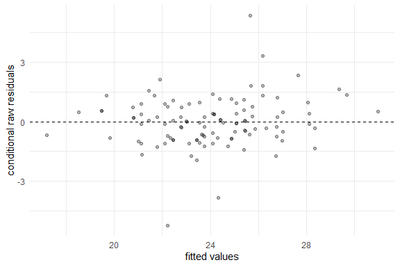
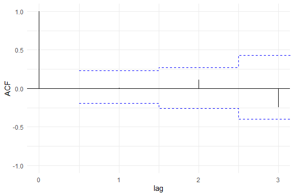
plot(fm1)
Several methods are available for SMSN and SMN objects, such as: print, summary, plot, fitted, residuals, and predict.
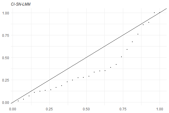
Some tools for goodness-of-fit assessment are also available, for example:

Furthermore, to fit a SMN-LMM one can use the following:
    fm2 <- smn.lmm(dat1,formFixed=distance ~ age,groupVar="Subject",quiet=T)
    summary(fm2)
#> Linear mixed models with distribution norm and dependency structure CI
#> Call:
#> smn.lmm(data = dat1, formFixed = distance ~ age, groupVar = "Subject",
#>     quiet = T)
#>
#> Distribution norm
#> Random effects: ~1
#> <environment: 0x000000001c19eb58>
#>   Estimated variance (D):
#>             (Intercept)
#> (Intercept)    4.289971
#>
#> Fixed effects: distance ~ age
#> with approximate confidence intervals
#>                  Value Std.error IC 95% lower IC 95% upper
#> (Intercept) 16.7611111 0.9928306   14.8151990    18.707023
#> age          0.6601852 0.0698073    0.5233654     0.797005
#>
#> Dependency structure: CI
#>   Estimate(s):
#>   sigma2
#> 2.025442
#>
#> Model selection criteria:
#>    logLik    AIC     BIC
#>  -221.695 451.39 462.118
#>
#> Number of observations: 108
#> Number of groups: 27
Now, for performing a LRT for testing if the skewness parameter is 0, one can use the following:
    lr.test(fm1,fm2)
#>
#> Model selection criteria:
#>       logLik     AIC     BIC
#> fm1 -221.658 453.316 466.726
#> fm2 -221.695 451.390 462.118
#>
#>     Likelihood-ratio Test
#>
#> chi-square statistics =  0.07388406
#> df =  1
#> p-value =  0.7857633
#>
#> The null hypothesis that both models represent the
#> data equally well is not rejected at level  0.05
For more examples, see help(smsn.lmm) and help(smn.lmm).