rsleep development version can be directly installed from Github using the devtools package.
devtools::install_github("boupetch/rsleep")Otherwise stable version can be downloaded and installed from CRAN [1] :
install.packages("rsleep")An example sleep record can be downloaded using the following code line. It contains full polysomnography data recorded over a whole night. Signals form sensors are stored in the European Data Format [2] (EDF) file, while events are stored in the Comma-Separated Values (CSV) file,
download.file("https://osf.io/57j2u/download", "15012016HD.edf", method="curl")

download.file("https://osf.io/h4ysj/download", "15012016HD.csv", method="curl")In rsleep, write_mdf() and read_mdf() functions are used to write and read records on disk. Files are converted from the EDF to Morpheo Data Format [3] (MDF). MDF is a simple, efficient and interoperable hierarchical file format for biological timeseries. The format supports raw signal and metadata storage. MDF uses binary files for signals and JSON for metadata.
if(!dir.exists("15012016HD")){
  events <- read_events_noxturnal("15012016HD.csv")

  write_mdf(edfPath = "15012016HD.edf",
            mdfPath = "15012016HD",
            channels = c("C3-M2", "ECG"),
            events = events)
}
events <- read_events_noxturnal("15012016HD.csv")

write_mdf(edfPath = "15012016HD.edf",
          mdfPath = "15012016HD",
          channels = c("C3-M2", "ECG"),
          events = events)
Once written on disk, MDF records can be read using the read_mdf() function. It quickly returns signals, events and metadata as a list.
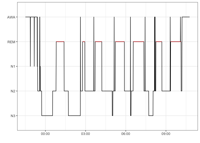
Hypnograms [4] can be plotted from stages data stored in a dataframe.

reference <- hypnogram(mdf$events)
reference <- reference[-nrow(reference),]

epochs <- epochs(signals = lapply(mdf$channels,function(x){x$signal}),
                 sRates = lapply(mdf$channels,function(x){x$metadata$sRate}),
                 resample = 200,
                 epoch = reference,
startTime = as.numeric(as.POSIXct(mdf$metadata$startTime)))Fourier transforms are computed over EEG during sleep since 1942 [5] . Spectrograms of whole night signals can be plotted using the spectrogram function.
spectrogram(signal = mdf$channels$`C3-M2`$signal,
            sRate = mdf$channels$`C3-M2`$metadata$sRate,
            startTime = as.POSIXct(mdf$metadata$startTime))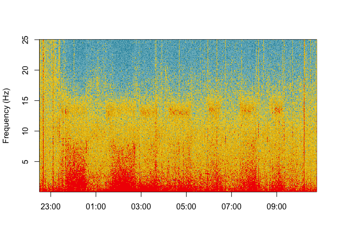
bands <- lapply(epochs,function(x){
  apply(x, 2, function(y){
    bands_power(bands = list(c(0.5,3.5),c(3.5,7.5),c(7.5,13),c(13,30)),
                signal = y, sRate = 200,
                broadband = c(0.5,30))
  })
})
c3m2 <- lapply(bands,function(x){
  unlist(x$`C3-M2`)
})
bands_df <- data.frame(matrix(unlist(c3m2), nrow=length(c3m2), byrow=TRUE))

colnames(bands_df) <- c("Delta","Theta","Alpha","Beta")
bands_df$stage <- reference$event
bands_df <- reshape2::melt(bands_df, id="stage")

summary(bands_df)
#>  stage       variable        value
#>  N3 :1024   Delta:1469   Min.   :0.004375
#>  N2 :2164   Theta:1469   1st Qu.:0.006235
#>  N1 :  36   Alpha:1469   Median :0.008367
#>  REM:1904   Beta :1469   Mean   :0.008254
#>  AWA: 748                3rd Qu.:0.009860
#>                          Max.   :0.014397
library(ggplot2)

pal <- c("#FF0000","#00A08A","#F98400","#5BBCD6")
ggplot(bands_df,aes(x=stage,y=value,fill=variable)) +
  geom_boxplot() + theme_bw() +
  scale_fill_manual(values = pal) +
  theme(legend.title = element_blank()) +
xlab("") + ylab("Normalized power") 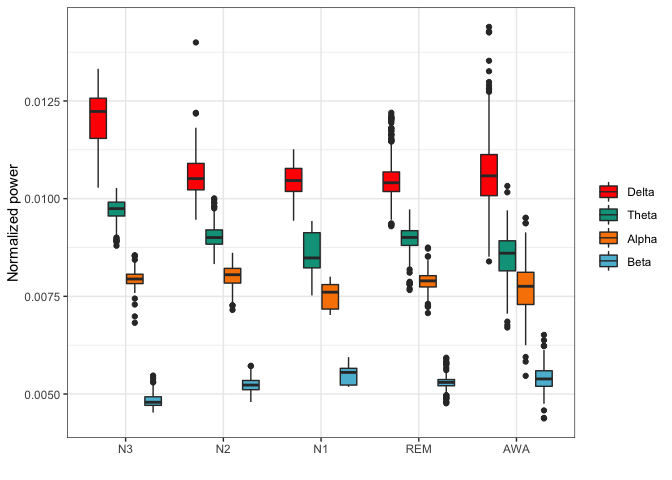
detect_rpeaks implements the first part of the Pan & Tompkins algorithm [6] to detect R peaks from an electrocardiogram (ECG) signal.
library(ggplot2)

sRate <- 200

ecg <- data.frame(Volts = example_ecg_200hz,
                  Seconds = c(1:length(example_ecg_200hz))/sRate)

rpeaks <- detect_rpeaks(example_ecg_200hz, sRate)

ggplot(ecg,
       aes(x = Seconds,
           y = Volts)) +
  geom_line() + theme_bw() +
  geom_vline(data.frame(p = rpeaks),
             mapping = aes(xintercept = p),
             linetype="dashed",color = "red")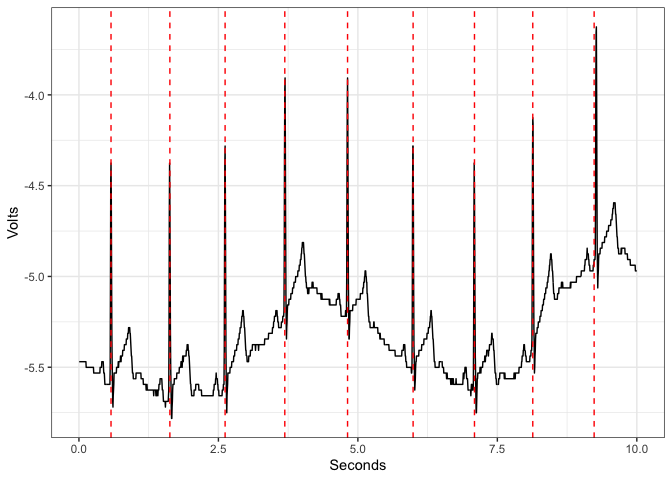
stages_stats function computes various statistics from the hypnogram.
rem_duration: Total duration of REM sleep in minutes.n1_duration: Total duration of N1 sleep in minutes.n2_duration: Total duration of N2 sleep in minutes.n3_duration: Total duration of N3 sleep in minutes.awa_duration: Total duration of wake in minutes.tts: Time To Sleep (N1+N2+N3+REM durations) in minutes.rem_tts: REM over TTS duration ratio.n3_tts: N3 over TTS duration ratio.n2_tts: N2 over TTS duration ratio.n1_tts: N1 over TTS duration ratio.tsp: Total Sleep Period.sleep_efficiency: Sleep Efficiency.sleep_latency: Sleep Latency.rem_latency: REM Sleep Latency.waso: Wake After Sleep Onset.
stages_stats(example_hypnogram_30s)
#> rem_duration  n1_duration  n2_duration  n3_duration awa_duration
#> 2.380000e+02 4.500000e+00 2.705000e+02 1.280000e+02 9.400000e+01
#>          tts      rem_tts       n1_tts       n2_tts       n3_tts
#> 6.410000e+02 3.712949e-01 7.020281e-03 4.219969e-01 1.996880e-01
#>      awa_tts          tsp   efficiency      latency   n1_latency
#> 1.466459e-01 7.360000e+02 8.709239e-01 2.200000e+01 0.000000e+00
#>   n2_latency   n3_latency  rem_latency         waso
#> 3.300000e+01 5.100000e+01 1.160000e+02 7.300000e+01[1] K. Hornik, The comprehensive r archive network, Wiley Interdisciplinary Reviews: Computational Statistics. 4 (2012) 394–398. https://cran.r-project.org/.
[2] B. Kemp, A. Värri, A.C. Rosa, K.D. Nielsen, J. Gade, A simple format for exchange of digitized polygraphic recordings, Electroencephalography and Clinical Neurophysiology. 82 (1992) 391–393. doi:10.1016/0013-4694(92)90009-7.
[3] P. Bouchequet, D. Jin, G. Solelhac, M. Chennaoui, D. Leger, Morpheo Data Format (MDF), un nouveau format de données simple, robuste et performant pour stocker et analyser les enregistrements de sommeil, Médecine Du Sommeil. 15 (2018) 48–49. doi:10.1016/j.msom.2018.01.130.
[4] AASM Scoring Manual - American Academy of Sleep Medicine, American Academy of Sleep Medicine Association for Sleep Clinicians and Researchers. (n.d.). https://aasm.org/clinical-resources/scoring-manual/.
[5] J.R. Knott, F.A. Gibbs, C.E. Henry, Fourier transforms of the electroencephalogram during sleep., Journal of Experimental Psychology. 31 (1942) 465–477. doi:10.1037/h0058545.
[6] J. Pan, W.J. Tompkins, A Real-Time QRS Detection Algorithm, IEEE Transactions on Biomedical Engineering. BME-32 (1985) 230–236. doi:10.1109/TBME.1985.325532.