
The rmdcev R package estimates and simulates multiple discrete-continuous extreme value (MDCEV) demand models with observed and unobserved individual heterogneity. Fixed parameter, latent class, and random parameter models can be estimated. These models are estimated using maximum likelihood or Bayesian estimation techniques and are implemented in Stan, which is a C++ package for performing full Bayesian inference (see http://mc-stan.org/). The package also includes functions for simulating demand and welfare outcomes from policy scenarios.
Development is in progress. Currently users can estimate the following models:
Under development
I recommend you first install rstan and C++ toolchain by following these steps:
https://github.com/stan-dev/rstan/wiki/RStan-Getting-Started
Once rstan is installed, you can install the released version of rmdcev from GitHub using devtools
if (!require(devtools)) {
  install.packages("devtools")
  library(devtools)
}
install_github("plloydsmith/rmdcev", build_vignettes = FALSE)
Depending on your computer set-up, you may need to adjust your Makevars file of the .R folder (usually in your computer user folder) to ensure the first two lines are
You can switch build_vignettes to TRUE but it will take a lot longer to install. If installation fails, please let me know by filing an issue.
For more details on the model specification and estimation:
Bhat, C.R. (2008) “The Multiple Discrete-Continuous Extreme Value (MDCEV) Model: Role of Utility Function Parameters, Identification Considerations, and Model Extensions.” Transportation Research Part B, 42(3): 274-303.
For more details on the welfare simulation:
Lloyd-Smith, P (2018). “A New Approach to Calculating Welfare Measures in Kuhn-Tucker Demand Models.” Journal of Choice Modeling, 26: 19-27
As an example, we can simulate some data using the Hybrid specification. In this example, we are simulating data for 1000 invdividuals and 10 non-numeraire alternatives.
library(pacman)
p_load(tidyverse, rmdcev)
model <- "hybrid"
nobs <- 1000
nalts <- 10
sim.data <- GenerateMDCEVData(model = model, nobs = nobs, nalts = nalts)
#> Checking data...
#> Data is good
Estimate model using MLE
mdcev_est <- mdcev(~ b1 + b2 + b3 + b4 + b5 + b6 + b7 + b8-1,
                   data = sim.data$data,
                   model = model,
                   algorithm = "MLE")
#> Using MLE to estimate MDCEV
#> Chain 1: Initial log joint probability = -9033.01
#> Chain 1:     Iter      log prob        ||dx||      ||grad||       alpha      alpha0  # evals  Notes
#> Chain 1:       19       -7445.3      0.511435       61.5753           1           1       26
#> Chain 1:     Iter      log prob        ||dx||      ||grad||       alpha      alpha0  # evals  Notes
#> Chain 1:       39      -7401.21      0.136793       26.4292           1           1       47
#> Chain 1:     Iter      log prob        ||dx||      ||grad||       alpha      alpha0  # evals  Notes
#> Chain 1:       59      -7395.55    0.00714899       6.06841       0.377       0.377       73
#> Chain 1:     Iter      log prob        ||dx||      ||grad||       alpha      alpha0  # evals  Notes
#> Chain 1:       79      -7395.22     0.0361296       3.24521           1           1       97
#> Chain 1:     Iter      log prob        ||dx||      ||grad||       alpha      alpha0  # evals  Notes
#> Chain 1:       99      -7395.13    0.00810581       2.07142      0.2972           1      118
#> Chain 1:     Iter      log prob        ||dx||      ||grad||       alpha      alpha0  # evals  Notes
#> Chain 1:      119      -7395.12    0.00245304      0.176321           1           1      141
#> Chain 1:     Iter      log prob        ||dx||      ||grad||       alpha      alpha0  # evals  Notes
#> Chain 1:      123      -7395.12   0.000199104       0.14664      0.3024           1      147
#> Chain 1: Optimization terminated normally:
#> Chain 1:   Convergence detected: relative gradient magnitude is below tolerance
Summarize results
summary(mdcev_est)
#> Model run using rmdcev for R, version 1.1.0
#> Estimation method                : MLE
#> Model type                       : hybrid specification
#> Number of classes                : 1
#> Number of individuals            : 499
#> Number of non-numeraire alts     : 10
#> Estimated parameters             : 20
#> LL                               : -7395.12
#> AIC                              : 14830.24
#> BIC                              : 14914.49
#> Standard errors calculated using : 50 MVN draws
#> Exit of MLE                      : successful convergence
#> Time taken (hh:mm:ss)            : 00:00:0.7
#>
#> Average consumption of non-numeraire alternatives:
#>     1     2     3     4     5     6     7     8     9    10
#> 15.43 19.36  8.32  6.25 20.97 31.69 34.04 35.23 14.96 10.91
#>
#> Parameter estimates --------------------------------
#>         Estimate Std.err z.stat
#> psi_b1    -4.512   0.738  -6.11
#> psi_b2     0.500   0.108   4.62
#> psi_b3     1.926   0.157  12.25
#> psi_b4    -1.579   0.172  -9.16
#> psi_b5     2.839   0.219  12.96
#> psi_b6    -1.787   0.173 -10.31
#> psi_b7     0.902   0.120   7.50
#> psi_b8     1.911   0.174  11.01
#> gamma1     1.925   0.557   3.46
#> gamma2     1.366   0.266   5.15
#> gamma3     1.548   0.383   4.05
#> gamma4     3.178   1.021   3.11
#> gamma5     1.661   0.318   5.22
#> gamma6     1.185   0.261   4.53
#> gamma7     1.672   0.311   5.37
#> gamma8     1.446   0.245   5.90
#> gamma9     1.388   0.252   5.50
#> gamma10    1.897   0.446   4.25
#> alpha1     0.514   0.037  13.72
#> scale      0.944   0.071  13.28
#> Note: Alpha parameter is equal for all alternatives.
Compare estimates to true values
parms_true <- tbl_df(sim.data$parms_true) %>%
    mutate(true = as.numeric(true))

output <- tbl_df(mdcev_est[["stan_fit"]][["theta_tilde"]]) %>%
                dplyr::select(-tidyselect::starts_with("log_like"),
                              -tidyselect::starts_with("sum_log_lik"))

names(output)[1:mdcev_est$parms_info$n_vars$n_parms_total] <- mdcev_est$parms_info$parm_names$all_names

output<- output %>%
        tibble::rowid_to_column("sim_id") %>%
        tidyr::gather(parms, value, -sim_id)

coefs <- output %>%
    mutate(parms = gsub("\\[|\\]", "", parms)) %>%
    group_by(parms) %>%
    summarise(mean = mean(value),
              sd = sd(value),
              zstat = mean / sd,
              cl_lo = quantile(value, 0.025),
              cl_hi = quantile(value, 0.975)) %>%
    left_join(parms_true, by = "parms") %>%
    print(n=200)
#> # A tibble: 20 x 7
#>    parms     mean     sd  zstat  cl_lo  cl_hi  true
#>    <chr>    <dbl>  <dbl>  <dbl>  <dbl>  <dbl> <dbl>
#>  1 alpha1   0.514 0.0375  13.7   0.427  0.575  0.5
#>  2 gamma1   1.93  0.557    3.46  1.22   3.26   1.96
#>  3 gamma10  1.90  0.446    4.25  1.19   2.86   1.84
#>  4 gamma2   1.37  0.266    5.15  0.971  1.88   1.03
#>  5 gamma3   1.55  0.383    4.05  0.926  2.49   1.75
#>  6 gamma4   3.18  1.02     3.11  1.75   5.05   1.99
#>  7 gamma5   1.66  0.318    5.22  1.17   2.31   1.54
#>  8 gamma6   1.18  0.261    4.53  0.831  1.77   1.26
#>  9 gamma7   1.67  0.311    5.37  1.24   2.31   1.51
#> 10 gamma8   1.45  0.245    5.90  1.01   1.92   1.42
#> 11 gamma9   1.39  0.252    5.50  0.923  1.88   1.54
#> 12 psi_b1  -4.51  0.738   -6.11 -6.19  -3.45  -5
#> 13 psi_b2   0.500 0.108    4.62  0.304  0.707  0.5
#> 14 psi_b3   1.93  0.157   12.2   1.68   2.24   2
#> 15 psi_b4  -1.58  0.172   -9.16 -1.92  -1.28  -1.5
#> 16 psi_b5   2.84  0.219   13.0   2.50   3.32   3
#> 17 psi_b6  -1.79  0.173  -10.3  -2.10  -1.46  -2
#> 18 psi_b7   0.902 0.120    7.50  0.679  1.12   1
#> 19 psi_b8   1.91  0.174   11.0   1.59   2.26   2
#> 20 scale    0.944 0.0711  13.3   0.833  1.11   1
Compare outputs using a figure
coefs %>%
    ggplot(aes(y = mean, x = true))  +
    geom_point(size=2) +
    geom_text(label=coefs$parms) +
    geom_abline(slope = 1) +
    geom_errorbar(aes(ymin=cl_lo,ymax=cl_hi,width=0.2))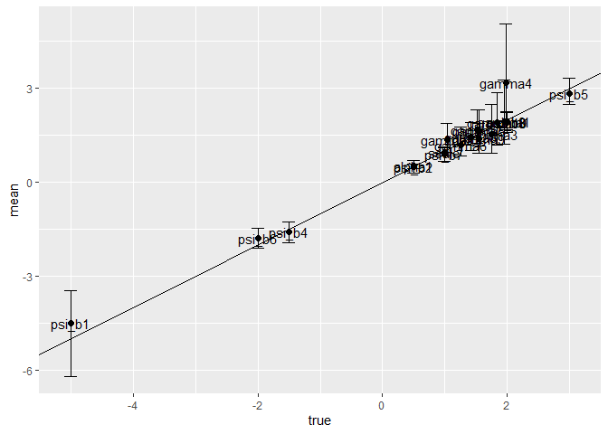
Create policy simulations (these are ‘no change’ policies with no effects)
npols <- 2 # Choose number of policies

policies<-  CreateBlankPolicies(npols, nalts, mdcev_est$stan_data[["dat_psi"]], price_change_only = TRUE)

df_sim <- PrepareSimulationData(mdcev_est, policies)
Simulate welfare changes
wtp <- mdcev.sim(df_sim$df_indiv,
                 df_common = df_sim$df_common,
                 sim_options = df_sim$sim_options,
                 cond_err = 1,
                 nerrs = 5,
                 sim_type = "welfare")
#> Using hybrid approach to simulation
#> Compiling simulation code
#> Simulating welfare...
#>
#> 1.50e+05simulations finished in0.03minutes.(71971per second)
summary(wtp)
#> # A tibble: 2 x 5
#>   policy      mean  std.dev `ci_lo2.5%` `ci_hi97.5%`
#>   <chr>      <dbl>    <dbl>       <dbl>        <dbl>
#> 1 policy1 1.09e-11 8.26e-11   -1.10e-10     1.47e-10
#> 2 policy2 1.09e-11 8.26e-11   -1.10e-10     1.47e-10