Version 1.0.15 built 2020-07-24 with R 4.0.2.
The library provides data sets (internal .rda and in CSV-format in /extdata/) which support users in a black-box performance qualification (PQ) of their software installations. Users can perform analysis of their own data imported from CSV- and Excel-files. The methods given by the EMA in Annex I for reference-scaling according to the EMA’s Guideline on the Investigation of Bioequivalence are implemented. Potential influence of outliers on the variability of the reference can be assessed by box plots of studentized and standardized residuals as suggested at a joint EGA/EMA workshop.
In full replicate designs the variability of test and reference treatments can be assessed by swT/swR and the upper confidence limit of σwT/σwR (required for the WHO’s approach for reference-scaling of AUC).
Called internally by functions method.A() and method.B(). A linear model of log-transformed pharmacokinetic (PK) responses and effects
sequence, subject(sequence), period
where all effects are fixed (i.e., ANOVA). Estimated by the function lm() of library stats.
modCVwR <- lm(log(PK) ~ sequence + subject%in%sequence + period,
                        data = data[data$treatment == "R", ])
modCVwT <- lm(log(PK) ~ sequence + subject%in%sequence + period,
data = data[data$treatment == "T", ])Called by function method.A(). A linear model of log-transformed PK responses and effects
sequence, subject(sequence), period, treatment
where all effects are fixed (i.e., ANOVA). Estimated by the function lm() of library stats.
Called by function method.B(). A linear model of log-transformed PK responses and effects
sequence, subject(sequence), period, treatment
where subject(sequence) is a random effect and all others are fixed.
Three options are provided
lme() of library nlme. Employs degrees of freedom equivalent to SAS’ DDFM=CONTAIN, Phoenix WinNonlin’s Degrees of Freedom Residual, STATISTICA’s GLM containment, and Stata’s dfm=anova. Implicitly preferred according to the EMA’s Q&A document and hence, the default of the function.lmer() of library lmerTest. Employs Satterthwaite’s approximation of the degrees of freedom method.B(..., option = 1) equivalent to SAS’ DDFM=SATTERTHWAITE, Phoenix WinNonlin’s Degrees of Freedom Satterthwaite, and Stata’s dfm=Satterthwaite. Note that this is the only available approximation in SPSS.lmer() of library lmerTest. Employs the Kenward-Roger approximation method.B(..., option = 3) equivalent to Stata’s dfm=Kenward Roger (EIM) and SAS’ DDFM=KENWARDROGER(FIRSTORDER) i.e., based on the expected information matrix. Note that SAS with DDFM=KENWARDROGER and JMP calculate Sattertwaite’s (sic) degrees of freedom and apply the Kackar-Harville correction i.e., based on the observed information matrix.Called by function ABE(). The model is identical to Method A. Conventional BE limits (80.00 – 125.00%) are employed by default. Tighter limits (90.00 – 111.11%) for narrow therapeutic index drugs (EMA) or wider limits (75.00 – 133.33%) for Cmax according to the guidelines of the Gulf Cooperation Council (Bahrain, Kuwait, Oman, Qatar, Saudi Arabia, United Arab Emirates) and South Africa can be specified.
TRTR | RTRT
TRRT | RTTR
TTRR | RRTT
TRTR | RTRT | TRRT | RTTR (confounded effects, not recommended)
TRRT | RTTR | TTRR | RRTT (confounded effects, not recommended)
TRT | RTR
TRR | RTT
TR | RT | TT | RR (Balaam’s design; not recommended due to poor power characteristics)
TRR | RTR | RRT
TRR | RTR (Extra-reference design; biased in the presence of period effects, not recommended)
Details about the reference datasets:
Results of the 30 reference datasets agree with ones obtained in SAS (9.4), Phoenix WinNonlin (6.4 – 8.1), STATISTICA (13), SPSS (22.0), Stata (15.0), and JMP (10.0.2).
library(replicateBE) # attach the library
res <- method.A(verbose = TRUE, details = TRUE, print = FALSE,
                data = rds01)
#
# Data set DS01: Method A by lm()
# -------------------------------
# Analysis of Variance Table
#
# Response: log(PK)
#                   Df   Sum Sq  Mean Sq  F value     Pr(>F)
# sequence           1   0.0077 0.007652  0.04783  0.8270958
# period             3   0.6984 0.232784  1.45494  0.2278285
# treatment          1   1.7681 1.768098 11.05095  0.0010405
# sequence:subject  75 214.1296 2.855061 17.84467 < 2.22e-16
# Residuals        217  34.7190 0.159995
#
# treatment T – R:
#   Estimate Std. Error    t value   Pr(>|t|)
# 0.14547400 0.04650870 3.12788000 0.00200215
# 217 Degrees of Freedom
cols <- c(12, 15:19)           # extract relevant columns
tmp  <- round(res[cols], 2)    # 2 decimal places acc. to GL
tmp  <- cbind(tmp, res[20:22]) # pass|fail
print(tmp, row.names = FALSE)
#  CVwR(%)  L(%)  U(%) CL.lo(%) CL.hi(%)  PE(%)   CI  GMR   BE
# 46.96 71.23 140.4 107.11 124.89 115.66 pass pass passres <- method.B(option = 3, ola = TRUE, verbose = TRUE, details = TRUE,
print = FALSE, data = rds01)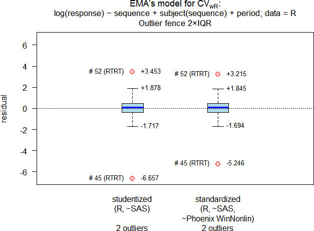
#
# Outlier analysis
#  (externally) studentized residuals
#  Limits (2×IQR whiskers): -1.717435, 1.877877
#  Outliers:
#  subject sequence  stud.res
#       45     RTRT -6.656940
#       52     RTRT  3.453122
#
#  standarized (internally studentized) residuals
#  Limits (2×IQR whiskers): -1.69433, 1.845333
#  Outliers:
#  subject sequence stand.res
#       45     RTRT -5.246293
#       52     RTRT  3.214663
#
# Data set DS01: Method B (option = 3) by lmer()
# ----------------------------------------------
# Response: log(PK)
# Type III Analysis of Variance Table with Kenward-Roger's method
#             Sum Sq  Mean Sq NumDF    DenDF F value    Pr(>F)
# sequence  0.001917 0.001917     1  74.9899 0.01198 0.9131528
# period    0.398065 0.132688     3 217.3875 0.82878 0.4792976
# treatment 1.579280 1.579280     1 217.2079 9.86432 0.0019197
#
# treatment T – R:
#   Estimate Std. Error    t value   Pr(>|t|)
#  0.1460900  0.0465140  3.1408000  0.0019197
# 217.208 Degrees of Freedom (equivalent to Stata’s dfm=Kenward Roger EIM)
cols <- c(25, 28:29, 17:19)    # extract relevant columns
tmp  <- round(res[cols], 2)    # 2 decimal places acc. to GL
tmp  <- cbind(tmp, res[30:32]) # pass|fail
print(tmp, row.names = FALSE)
#  CVwR.rec(%) L.rec(%) U.rec(%) CL.lo(%) CL.hi(%)  PE(%) CI.rec GMR.rec BE.rec
# 32.16 78.79 126.93 107.17 124.97 115.73 pass pass passres <- ABE(verbose = TRUE, theta1 = 0.90, details = TRUE,
print = FALSE, data = rds05)
#
# Data set DS05: ABE by lm()
# --------------------------
# Analysis of Variance Table
#
# Response: log(PK)
# Df Sum Sq Mean Sq F value Pr(>F)
# sequence 1 0.092438 0.0924383 6.81025 0.0109629
# period 3 0.069183 0.0230609 1.69898 0.1746008
# treatment 1 0.148552 0.1485523 10.94435 0.0014517
# sequence:subject 24 2.526550 0.1052729 7.75581 4.0383e-12
# Residuals 74 1.004433 0.0135734
#
# treatment T – R:
# Estimate Std. Error t value Pr(>|t|)
# 0.07558800 0.02284850 3.30822000 0.00145167
# 74 Degrees of Freedom
cols <- c(13:17) # extract relevant columns
tmp <- round(res[cols], 2) # 2 decimal places acc. to GL
tmp <- cbind(tmp, res[18]) # pass|fail
print(tmp, row.names=FALSE)
# BE.lo(%) BE.hi(%) CL.lo(%) CL.hi(%) PE(%) BE
# 90 111.11 103.82 112.04 107.85 failThe package requires R ≥ 3.5.0; for the Kenward-Roger approximation method.B(..., option = 3) R ≥ 3.6.0 is required.
To use the development version, please install the released version from CRAN first to get its dependencies right (readxl ≥ 1.0.0, PowerTOST ≥ 1.3.3, lmerTest, nlme, pbkrtest).
You need tools for building R packages from sources on your machine. For Windows users:
devtools and build the development version by:install.packages("devtools", repos = "https://cloud.r-project.org/")
devtools::install_github("Helmut01/replicateBE")Package offered for Use without any Guarantees and Absolutely No Warranty. No Liability is accepted for any Loss and Risk to Public Health Resulting from Use of this R-Code.