


{readabs} helps you easily download, import, and tidy time series data from the Australian Bureau of Statistics within R. This saves you time manually downloading and tediously tidying time series data and allows you to spend more time on your analysis.
Github issues containing error reports or feature requests are welcome. Alternatively you can email the package maintainer at mattcowgill at gmail dot com.
Install the latest CRAN version of {readabs} with:
You can install the developer version of {readabs} from GitHub with:
# if you don't have devtools installed, first run:
# install.packages("devtools")
devtools::install_github("mattcowgill/readabs")There is one key function in {readabs}. It is read_abs(), which downloads, imports, and tidies time series data from the ABS website.
There are some other functions you may find useful.
read_abs_local() imports and tidies time series data from ABS spreadsheets stored on a local drive.separate_series() splits the series column of a tidied ABS time series spreadsheet into multiple columns, reducing the manual wrangling that’s needed to work with the data.Both read_abs() and read_abs_local() return a single tidy data frame (tibble).
To download all the time series data from an ABS catalogue number to your disk, and import the data to R as a single tidy data frame, use read_abs().
First we’ll load {readabs} and the {tidyverse}:
library(readabs)
#> Environment variable 'R_READABS_PATH' is unset. Downloaded files will be saved in a temporary directory.
#> You can set 'R_READABS_PATH' at any time. To set it for the rest of this session, use
#>  Sys.setenv(R_READABS_PATH = <path>)
library(tidyverse)
#> ── Attaching packages ───────────────────────────────────────────────────────────────────────────────────────────────── tidyverse 1.3.0 ──
#> ✔ ggplot2 3.2.1     ✔ purrr   0.3.3
#> ✔ tibble  2.1.3     ✔ dplyr   0.8.3
#> ✔ tidyr   1.0.0     ✔ stringr 1.4.0
#> ✔ readr   1.3.1     ✔ forcats 0.4.0
#> ── Conflicts ──────────────────────────────────────────────────────────────────────────────────────────────────── tidyverse_conflicts() ──
#> ✖ dplyr::filter() masks stats::filter()
#> ✖ dplyr::lag()    masks stats::lag()
Now we’ll create one data frame that contains all the time series data from the Wage Price Index, catalogue number 6345.0:
all_wpi <- read_abs("6345.0")
#> Finding filenames for tables corresponding to ABS catalogue 6345.0
#> Attempting to download files from catalogue 6345.0, Wage Price Index, Australia
#> Extracting data from downloaded spreadsheets
#> Tidying data from imported ABS spreadsheets
This is what it looks like:
str(all_wpi)
#> Classes 'tbl_df', 'tbl' and 'data.frame':    56819 obs. of  12 variables:
#>  $ table_no        : chr  "634501" "634501" "634501" "634501" ...
#>  $ sheet_no        : chr  "Data1" "Data1" "Data1" "Data1" ...
#>  $ table_title     : chr  "Table 1. Total Hourly Rates of Pay Excluding Bonuses: Sector, Original, Seasonally Adjusted and Trend" "Table 1. Total Hourly Rates of Pay Excluding Bonuses: Sector, Original, Seasonally Adjusted and Trend" "Table 1. Total Hourly Rates of Pay Excluding Bonuses: Sector, Original, Seasonally Adjusted and Trend" "Table 1. Total Hourly Rates of Pay Excluding Bonuses: Sector, Original, Seasonally Adjusted and Trend" ...
#>  $ date            : Date, format: "1997-09-01" "1997-12-01" ...
#>  $ series          : chr  "Quarterly Index ;  Total hourly rates of pay excluding bonuses ;  Australia ;  Private ;  All industries ;" "Quarterly Index ;  Total hourly rates of pay excluding bonuses ;  Australia ;  Private ;  All industries ;" "Quarterly Index ;  Total hourly rates of pay excluding bonuses ;  Australia ;  Private ;  All industries ;" "Quarterly Index ;  Total hourly rates of pay excluding bonuses ;  Australia ;  Private ;  All industries ;" ...
#>  $ value           : num  67.4 67.9 68.5 68.8 69.6 70 70.4 70.8 71.5 71.9 ...
#>  $ series_type     : chr  "Original" "Original" "Original" "Original" ...
#>  $ data_type       : chr  "INDEX" "INDEX" "INDEX" "INDEX" ...
#>  $ collection_month: chr  "3" "3" "3" "3" ...
#>  $ frequency       : chr  "Quarter" "Quarter" "Quarter" "Quarter" ...
#>  $ series_id       : chr  "A2603039T" "A2603039T" "A2603039T" "A2603039T" ...
#>  $ unit            : chr  "Index Numbers" "Index Numbers" "Index Numbers" "Index Numbers" ...
It only takes you a few lines of code to make a graph from your data:
all_wpi %>%
  filter(series == "Percentage Change From Corresponding Quarter of Previous Year ;  Australia ;  Total hourly rates of pay excluding bonuses ;  Private and Public ;  All industries ;",
         !is.na(value)) %>%
  ggplot(aes(x = date, y = value, col = series_type)) +
  geom_line() +
  theme_minimal() +
  labs(y = "Annual wage growth (per cent)")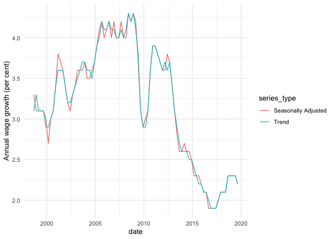
In the example above we downloaded all the time series from a catalogue number. This will often be overkill. If you know the data you need is in a particular table, you can just get that table like this:
wpi_t1 <- read_abs("6345.0", tables = 1)
#> Warning in read_abs("6345.0", tables = 1): `tables` was provided, yet
#> `check_local = TRUE` and fst files are available so `tables` will be ignored.
If you want multiple tables, but not the whole catalogue, that’s easy too:
wpi_t1_t5 <- read_abs("6345.0", tables = c("1", "5a"))
#> Warning in read_abs("6345.0", tables = c("1", "5a")): `tables` was provided, yet
#> `check_local = TRUE` and fst files are available so `tables` will be ignored.
In most cases, the series column will contain multiple components, separated by ‘;’. The separate_series() function can help wrangling this column.
For more examples, please see the readabs vignette (run browseVignettes("readabs")).
In 0.4.3,
read_abs() checks to see if you are connected to the internet, and can connect to the ABS website, before trying to download data. The method used for checking connectivity has been improved, to make the function compatible with a broader range of IT environments. Thanks to Oscar Lane for noticing the issue and proposing a fix.In 0.4.2,
read_abs() is now set by an environment variable, rather than defaulting to ‘data/ABS’. If the variable is not set, downloaded files will be stored in a temporary directory. Thanks to Hugh Parsonage for the idea and implementation. See ?read_abs for more information.In 0.4.1,
separate_series() function gained a remove_nas argument - thanks to Sam Gow for the suggestion. This makes tidying data easier.In 0.4.0,
separate_series() function was added, to be used in conjunction with read_abs() to help tidy data (thanks to David Diviny).read_cpi() convenience function was added; it returns a tibble containing dates and CPI index numbers.read_abs() function now has an optional series_id argument, allowing users to get individual time series by using the unique identifiers given to them by the ABS.read_abs() function now has a retain_files argument (TRUE by default); by setting this to FALSE, downloaded spreadsheets will be stored in a temporary directory![]()
We’re pleased to be included in a list of software that can be used to work with official statistics.
From version 0.3.0, readabs gained significant new functionality and the package changed substantially. Pre-0.3.0 functions still work, but read_abs_data() is deprecated. The behaviour of read_abs_metadata() has changed and the function is deprecated. The old version of readabs is available in the 0.2.9 branch on Github.