![]()


The prioritizr R package uses integer linear programming (ILP) techniques to provide a flexible interface for building and solving conservation planning problems. It supports a broad range of objectives, constraints, and penalties that can be used to custom-tailor conservation planning problems to the specific needs of a conservation planning exercise. Once built, conservation planning problems can be solved using a variety of commercial and open-source exact algorithm solvers. In contrast to the algorithms conventionally used to solve conservation problems, such as heuristics or simulated annealing, the exact algorithms used here are guaranteed to find optimal solutions. Furthermore, conservation problems can be constructed to optimize the spatial allocation of different management actions or zones, meaning that conservation practitioners can identify solutions that benefit multiple stakeholders. Finally, this package has the functionality to read input data formatted for the Marxan conservation planning program, and find much cheaper solutions in a much shorter period of time than Marxan.
The latest official version of the prioritizr R package can be installed from the Comprehensive R Archive Network (CRAN) using the following R code.
Alternatively, the latest development version can be installed from GitHub using the following code. Please note that while developmental versions may contain additional features not present in the official version, they may also contain coding errors.
Please cite the prioritizr R package when using it in publications. To cite the latest official version, please use:
Hanson JO, Schuster R, Morrell N, Strimas-Mackey M, Watts ME, Arcese P, Bennett J, Possingham HP (2020). prioritizr: Systematic Conservation Prioritization in R. R package version 5.0.2. Available at https://CRAN.R-project.org/package=prioritizr.
Alternatively, to cite the latest development version, please use:
Hanson JO, Schuster R, Morrell N, Strimas-Mackey M, Watts ME, Arcese P, Bennett J, Possingham HP (2020). prioritizr: Systematic Conservation Prioritization in R. R package version 5.0.2. Available at https://github.com/prioritizr/prioritizr.
Additionally, we keep a record of publications that use the prioritizr R package. If you use this package in any reports or publications, please file an issue on GitHub so we can add it to the record.
Here we will provide a short example showing how the prioritizr R package can be used to build and solve conservation problems. For brevity, we will use one of the built-in simulated data sets that is distributed with the package. First, we will load the prioritizr R package.
We will use the sim_pu_polygons object to represent our planning units. Although the prioritizr R can support many different types of planning unit data, here our planning units are represented as polygons in a spatial vector format (i.e. SpatialPolygonsDataFrame). Each polygon represents a different planning unit and we have 90 planning units in total. The attribute table associated with this data set contains information describing the acquisition cost of each planning (“cost” column), and a value indicating if the unit is already located in protected area (“locked_in” column). Let’s explore the planning unit data.
# load planning unit data
data(sim_pu_polygons)

# show the first 6 rows in the attribute table
head(sim_pu_polygons@data)
## cost locked_in locked_out
## 1 215.8638 FALSE FALSE
## 2 212.7823 FALSE FALSE
## 3 207.4962 FALSE FALSE
## 4 208.9322 FALSE TRUE
## 5 214.0419 FALSE FALSE
## 6 213.7636 FALSE FALSE# plot the planning units and color them according to acquisition cost
spplot(sim_pu_polygons, "cost", main = "Planning unit cost",
xlim = c(-0.1, 1.1), ylim = c(-0.1, 1.1))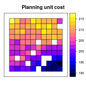
# plot the planning units and show which planning units are inside protected
# areas (colored in yellow)
spplot(sim_pu_polygons, "locked_in", main = "Planning units in protected areas",
       xlim = c(-0.1, 1.1), ylim = c(-0.1, 1.1))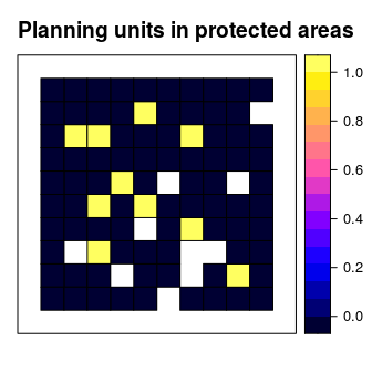
Conservation features are represented using a stack of raster data (i.e. RasterStack objects). A RasterStack represents a collection of RasterLayers with the same spatial properties (i.e. spatial extent, coordinate system, dimensionality, and resolution). Each RasterLayer in the stack describes the distribution of a conservation feature.
In our example, the sim_features object is a RasterStack object that contains 5 layers. Each RasterLayer describes the distribution of a species. Specifically, the pixel values denote the proportion of suitable habitat across different areas inside the study area. For a given layer, pixels with a value of one are comprised entirely of suitable habitat for the feature, and pixels with a value of zero contain no suitable habitat.
# load feature data
data(sim_features)

# plot the distribution of suitable habitat for each feature
plot(sim_features, main = paste("Feature", seq_len(nlayers(sim_features))),
     nr = 2)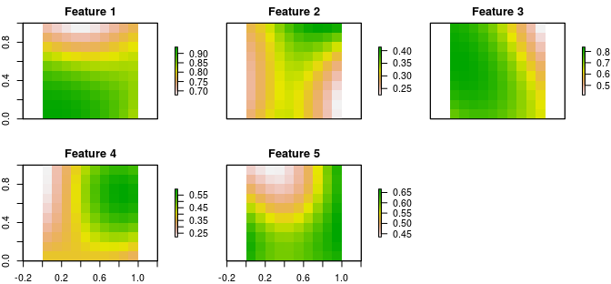
Let’s say that we want to develop a reserve network that will secure 15% of the distribution for each feature in the study area for minimal cost. In this planning scenario, we can either purchase all of the land inside a given planning unit, or none of the land inside a given planning unit. Thus we will create a new problem that will use a minimum set objective (add_min_set_objective), with relative targets of 15% (add_relative_targets), binary decisions (add_binary_decisions), and specify that we want to want optimal solutions from the best solver installed on our system (add_default_solver).
# create problem
p1 <- problem(sim_pu_polygons, features = sim_features,
              cost_column = "cost") %>%
      add_min_set_objective() %>%
      add_relative_targets(0.15) %>%
      add_binary_decisions() %>%
      add_default_solver(gap = 0)
After we have built a problem, we can solve it to obtain a solution. Since we have not specified the method used to solve the problem, prioritizr will automatically use the best solver currently installed. It is strongly encouraged to install the Gurobi software suite and the gurobi R package to solve problems quickly, for more information on this please refer to the Gurobi Installation Guide
## Gurobi Optimizer version 9.0.2 build v9.0.2rc0 (linux64)
## Optimize a model with 5 rows, 90 columns and 450 nonzeros
## Model fingerprint: 0x8f50132f
## Variable types: 0 continuous, 90 integer (90 binary)
## Coefficient statistics:
##   Matrix range     [2e-01, 9e-01]
##   Objective range  [2e+02, 2e+02]
##   Bounds range     [1e+00, 1e+00]
##   RHS range        [4e+00, 1e+01]
## Found heuristic solution: objective 3139.8880309
## Presolve time: 0.00s
## Presolved: 5 rows, 90 columns, 450 nonzeros
## Variable types: 0 continuous, 90 integer (90 binary)
## Presolved: 5 rows, 90 columns, 450 nonzeros
##
##
## Root relaxation: objective 2.611170e+03, 13 iterations, 0.00 seconds
##
##     Nodes    |    Current Node    |     Objective Bounds      |     Work
##  Expl Unexpl |  Obj  Depth IntInf | Incumbent    BestBd   Gap | It/Node Time
##
##      0     0 2611.17006    0    4 3139.88803 2611.17006  16.8%     -    0s
## H    0     0                    2780.0314635 2611.17006  6.07%     -    0s
##      0     0 2611.74321    0    5 2780.03146 2611.74321  6.05%     -    0s
## H    0     0                    2750.8323723 2611.74321  5.06%     -    0s
##      0     0 2611.83195    0    6 2750.83237 2611.83195  5.05%     -    0s
##      0     0 2611.88195    0    7 2750.83237 2611.88195  5.05%     -    0s
## H    0     0                    2747.3774616 2611.88195  4.93%     -    0s
##      0     0 2611.94509    0    7 2747.37746 2611.94509  4.93%     -    0s
##      0     0 2611.95916    0    8 2747.37746 2611.95916  4.93%     -    0s
##      0     0 2611.98750    0    8 2747.37746 2611.98750  4.93%     -    0s
##      0     0 2612.13884    0    9 2747.37746 2612.13884  4.92%     -    0s
##      0     0 2612.17380    0    9 2747.37746 2612.17380  4.92%     -    0s
##      0     0 2612.35043    0   10 2747.37746 2612.35043  4.91%     -    0s
##      0     0 2612.36452    0   10 2747.37746 2612.36452  4.91%     -    0s
##      0     0 2612.42169    0    9 2747.37746 2612.42169  4.91%     -    0s
##      0     0 2612.45702    0    9 2747.37746 2612.45702  4.91%     -    0s
##      0     0 2612.47359    0   10 2747.37746 2612.47359  4.91%     -    0s
##      0     0 2612.47538    0   11 2747.37746 2612.47538  4.91%     -    0s
##      0     0 2612.48905    0    9 2747.37746 2612.48905  4.91%     -    0s
##      0     0 2612.52192    0    9 2747.37746 2612.52192  4.91%     -    0s
##      0     0 2612.52381    0   10 2747.37746 2612.52381  4.91%     -    0s
##      0     0 2612.57002    0    9 2747.37746 2612.57002  4.91%     -    0s
##      0     0 2612.57755    0   10 2747.37746 2612.57755  4.91%     -    0s
##      0     0 2612.59388    0   10 2747.37746 2612.59388  4.91%     -    0s
##      0     0 2612.63348    0    9 2747.37746 2612.63348  4.90%     -    0s
##      0     0 2612.64156    0   10 2747.37746 2612.64156  4.90%     -    0s
##      0     0 2612.66269    0   10 2747.37746 2612.66269  4.90%     -    0s
##      0     0 2612.72195    0    9 2747.37746 2612.72195  4.90%     -    0s
##      0     0 2612.78753    0   10 2747.37746 2612.78753  4.90%     -    0s
##      0     0 2612.78891    0   11 2747.37746 2612.78891  4.90%     -    0s
##      0     0 2613.13568    0    7 2747.37746 2613.13568  4.89%     -    0s
##      0     0 2613.22338    0    8 2747.37746 2613.22338  4.88%     -    0s
##      0     0 2613.34297    0    9 2747.37746 2613.34297  4.88%     -    0s
##      0     0 2613.51894    0   10 2747.37746 2613.51894  4.87%     -    0s
##      0     0 2613.52981    0   10 2747.37746 2613.52981  4.87%     -    0s
##      0     0 2613.62584    0   11 2747.37746 2613.62584  4.87%     -    0s
##      0     0 2613.62990    0   10 2747.37746 2613.62990  4.87%     -    0s
##      0     0 2613.64411    0   11 2747.37746 2613.64411  4.87%     -    0s
##      0     0 2613.70527    0   10 2747.37746 2613.70527  4.87%     -    0s
##      0     0 2613.74931    0   10 2747.37746 2613.74931  4.86%     -    0s
##      0     0 2613.75935    0   11 2747.37746 2613.75935  4.86%     -    0s
##      0     0 2613.78321    0   10 2747.37746 2613.78321  4.86%     -    0s
##      0     0 2613.85241    0   10 2747.37746 2613.85241  4.86%     -    0s
##      0     0 2613.85382    0   11 2747.37746 2613.85382  4.86%     -    0s
##      0     0 2613.85510    0   11 2747.37746 2613.85510  4.86%     -    0s
##      0     0 2613.85824    0   12 2747.37746 2613.85824  4.86%     -    0s
##      0     0 2613.86743    0   12 2747.37746 2613.86743  4.86%     -    0s
##      0     0 2613.89542    0   12 2747.37746 2613.89542  4.86%     -    0s
##      0     0 2613.90080    0   13 2747.37746 2613.90080  4.86%     -    0s
##      0     0 2613.90780    0   14 2747.37746 2613.90780  4.86%     -    0s
##      0     0 2613.91321    0   14 2747.37746 2613.91321  4.86%     -    0s
##      0     0 2613.93526    0   12 2747.37746 2613.93526  4.86%     -    0s
##      0     0 2613.93676    0   13 2747.37746 2613.93676  4.86%     -    0s
##      0     0 2614.07265    0   12 2747.37746 2614.07265  4.85%     -    0s
##      0     0 2614.12054    0   12 2747.37746 2614.12054  4.85%     -    0s
##      0     0 2614.15681    0   12 2747.37746 2614.15681  4.85%     -    0s
##      0     0 2614.15970    0   13 2747.37746 2614.15970  4.85%     -    0s
##      0     0 2614.26936    0   12 2747.37746 2614.26936  4.84%     -    0s
##      0     0 2614.28046    0   12 2747.37746 2614.28046  4.84%     -    0s
##      0     0 2614.30152    0   11 2747.37746 2614.30152  4.84%     -    0s
##      0     0 2614.30559    0   12 2747.37746 2614.30559  4.84%     -    0s
##      0     0 2614.31022    0   13 2747.37746 2614.31022  4.84%     -    0s
##      0     0 2614.32003    0   12 2747.37746 2614.32003  4.84%     -    0s
##      0     0 2614.32230    0   13 2747.37746 2614.32230  4.84%     -    0s
##      0     0 2614.32331    0   13 2747.37746 2614.32331  4.84%     -    0s
##      0     2 2614.33358    0   13 2747.37746 2614.33358  4.84%     -    0s
## H 7050   989                    2627.6389306 2618.95150  0.33%   1.8    0s
##
## Cutting planes:
##   Gomory: 5
##   Cover: 5
##   MIR: 46
##   StrongCG: 25
##   Flow cover: 2
##
## Explored 31196 nodes (83170 simplex iterations) in 2.60 seconds
## Thread count was 1 (of 4 available processors)
##
## Solution count 5: 2627.64 2747.38 2750.83 ... 3139.89
##
## Optimal solution found (tolerance 0.00e+00)
## Best objective 2.627638930618e+03, best bound 2.627638930618e+03, gap 0.0000%## solution_1
## 2627.639## solution_1
## 2.596609## solution_1
## "OPTIMAL"# plot the solution
spplot(s1, "solution_1", main = "Solution", at = c(0, 0.5, 1.1),
col.regions = c("grey90", "darkgreen"), xlim = c(-0.1, 1.1),
ylim = c(-0.1, 1.1))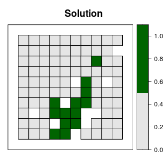
Although this solution adequately conserves each feature, it is inefficient because it does not consider the fact some of the planning units are already inside protected areas. Since our planning unit data contains information on which planning units are already inside protected areas (in the "locked_in" column of the attribute table), we can add constraints to ensure they are prioritized in the solution (add_locked_in_constraints).
# create new problem with locked in constraints added to it
p2 <- p1 %>%
      add_locked_in_constraints("locked_in")

# solve the problem
s2 <- solve(p2)
## Gurobi Optimizer version 9.0.2 build v9.0.2rc0 (linux64)
## Optimize a model with 5 rows, 90 columns and 450 nonzeros
## Model fingerprint: 0xb2af8965
## Variable types: 0 continuous, 90 integer (90 binary)
## Coefficient statistics:
## Matrix range [2e-01, 9e-01]
## Objective range [2e+02, 2e+02]
## Bounds range [1e+00, 1e+00]
## RHS range [4e+00, 1e+01]
## Found heuristic solution: objective 3027.6970854
## Presolve removed 0 rows and 10 columns
## Presolve time: 0.00s
## Presolved: 5 rows, 80 columns, 400 nonzeros
## Variable types: 0 continuous, 80 integer (80 binary)
## Presolved: 5 rows, 80 columns, 400 nonzeros
##
##
## Root relaxation: objective 2.754438e+03, 12 iterations, 0.00 seconds
##
## Nodes | Current Node | Objective Bounds | Work
## Expl Unexpl | Obj Depth IntInf | Incumbent BestBd Gap | It/Node Time
##
## 0 0 2754.43796 0 4 3027.69709 2754.43796 9.03% - 0s
## H 0 0 2839.1208991 2754.43796 2.98% - 0s
## 0 0 2835.61695 0 3 2839.12090 2835.61695 0.12% - 0s
## 0 0 2835.66921 0 3 2839.12090 2835.66921 0.12% - 0s
## 0 0 2835.66921 0 3 2839.12090 2835.66921 0.12% - 0s
## 0 0 2835.66921 0 3 2839.12090 2835.66921 0.12% - 0s
## 0 0 2835.93929 0 4 2839.12090 2835.93929 0.11% - 0s
## 0 0 2836.06802 0 4 2839.12090 2836.06802 0.11% - 0s
## 0 0 2836.33448 0 5 2839.12090 2836.33448 0.10% - 0s
## 0 0 2836.49814 0 5 2839.12090 2836.49814 0.09% - 0s
## 0 0 2836.77716 0 6 2839.12090 2836.77716 0.08% - 0s
## 0 0 2836.82966 0 7 2839.12090 2836.82966 0.08% - 0s
## 0 0 2836.87897 0 7 2839.12090 2836.87897 0.08% - 0s
## 0 0 2836.88941 0 7 2839.12090 2836.88941 0.08% - 0s
## 0 0 2836.89042 0 8 2839.12090 2836.89042 0.08% - 0s
## 0 0 2836.99962 0 7 2839.12090 2836.99962 0.07% - 0s
## 0 0 2837.08985 0 7 2839.12090 2837.08985 0.07% - 0s
## 0 0 2837.24552 0 6 2839.12090 2837.24552 0.07% - 0s
## 0 0 2837.31750 0 9 2839.12090 2837.31750 0.06% - 0s
## 0 0 2837.36426 0 10 2839.12090 2837.36426 0.06% - 0s
## 0 0 2837.39901 0 11 2839.12090 2837.39901 0.06% - 0s
## 0 0 2837.50764 0 10 2839.12090 2837.50764 0.06% - 0s
## 0 0 2837.51431 0 10 2839.12090 2837.51431 0.06% - 0s
## 0 0 2837.53639 0 9 2839.12090 2837.53639 0.06% - 0s
## 0 0 2837.53849 0 10 2839.12090 2837.53849 0.06% - 0s
## 0 0 2837.72116 0 8 2839.12090 2837.72116 0.05% - 0s
## 0 0 2837.76058 0 8 2839.12090 2837.76058 0.05% - 0s
## 0 0 2837.76433 0 9 2839.12090 2837.76433 0.05% - 0s
## 0 0 2837.77226 0 9 2839.12090 2837.77226 0.05% - 0s
## 0 0 2837.78842 0 10 2839.12090 2837.78842 0.05% - 0s
## 0 0 2837.82220 0 9 2839.12090 2837.82220 0.05% - 0s
## 0 0 2837.82524 0 10 2839.12090 2837.82524 0.05% - 0s
## 0 0 2837.87512 0 9 2839.12090 2837.87512 0.04% - 0s
## 0 0 2837.88038 0 10 2839.12090 2837.88038 0.04% - 0s
## 0 0 2837.95407 0 9 2839.12090 2837.95407 0.04% - 0s
## 0 0 2837.96355 0 9 2839.12090 2837.96355 0.04% - 0s
## 0 0 2838.04745 0 7 2839.12090 2838.04745 0.04% - 0s
## H 0 0 2838.2640999 2838.04745 0.01% - 0s
## 0 0 2838.12770 0 5 2838.26410 2838.12770 0.00% - 0s
##
## Cutting planes:
## MIR: 7
## StrongCG: 3
##
## Explored 1 nodes (95 simplex iterations) in 0.02 seconds
## Thread count was 1 (of 4 available processors)
##
## Solution count 3: 2838.26 2839.12 3027.7
##
## Optimal solution found (tolerance 0.00e+00)
## Best objective 2.838264099909e+03, best bound 2.838264099909e+03, gap 0.0000%# plot the solution
spplot(s2, "solution_1", main = "Solution", at = c(0, 0.5, 1.1),
col.regions = c("grey90", "darkgreen"), xlim = c(-0.1, 1.1),
ylim = c(-0.1, 1.1))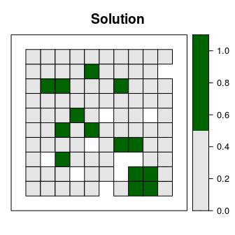
This solution is an improvement over the previous solution. However, it is also highly fragmented. As a consequence, this solution may be associated with increased management costs and the species in this scenario may not benefit substantially from this solution due to edge effects. We can further modify the problem by adding penalties that punish overly fragmented solutions (add_boundary_penalties). Here we will use a penalty factor of 300 (i.e. boundary length modifier; BLM), and an edge factor of 50% so that planning units that occur outer edge of the study area are not overly penalized.
# create new problem with boundary penalties added to it
p3 <- p2 %>%
      add_boundary_penalties(penalty = 300, edge_factor = 0.5)

# solve the problem
s3 <- solve(p3)
## Gurobi Optimizer version 9.0.2 build v9.0.2rc0 (linux64)
## Optimize a model with 293 rows, 234 columns and 1026 nonzeros
## Model fingerprint: 0x517c913c
## Variable types: 0 continuous, 234 integer (234 binary)
## Coefficient statistics:
## Matrix range [2e-01, 1e+00]
## Objective range [6e+01, 3e+02]
## Bounds range [1e+00, 1e+00]
## RHS range [4e+00, 1e+01]
## Found heuristic solution: objective 19567.196992
## Found heuristic solution: objective 4347.6970854
## Presolve removed 72 rows and 46 columns
## Presolve time: 0.00s
## Presolved: 221 rows, 188 columns, 832 nonzeros
## Variable types: 0 continuous, 188 integer (188 binary)
## Presolved: 221 rows, 188 columns, 832 nonzeros
##
##
## Root relaxation: objective 3.862929e+03, 120 iterations, 0.00 seconds
##
## Nodes | Current Node | Objective Bounds | Work
## Expl Unexpl | Obj Depth IntInf | Incumbent BestBd Gap | It/Node Time
##
## 0 0 3862.92934 0 65 4347.69709 3862.92934 11.1% - 0s
## H 0 0 4091.9945792 3862.92934 5.60% - 0s
## H 0 0 4058.7498291 3862.92934 4.82% - 0s
## H 0 0 3951.7528370 3862.92934 2.25% - 0s
## 0 0 3889.41281 0 41 3951.75284 3889.41281 1.58% - 0s
## H 0 0 3939.6015361 3889.41281 1.27% - 0s
## 0 0 3892.64817 0 63 3939.60154 3892.64817 1.19% - 0s
## 0 0 3896.53163 0 85 3939.60154 3896.53163 1.09% - 0s
## 0 0 3910.26013 0 8 3939.60154 3910.26013 0.74% - 0s
## 0 0 3910.58042 0 9 3939.60154 3910.58042 0.74% - 0s
## 0 0 3915.80407 0 6 3939.60154 3915.80407 0.60% - 0s
## 0 0 3934.87486 0 4 3939.60154 3934.87486 0.12% - 0s
##
## Cutting planes:
## GUB cover: 2
##
## Explored 1 nodes (217 simplex iterations) in 0.03 seconds
## Thread count was 1 (of 4 available processors)
##
## Solution count 6: 3939.6 3951.75 4058.75 ... 19567.2
##
## Optimal solution found (tolerance 0.00e+00)
## Best objective 3.939601536145e+03, best bound 3.939601536145e+03, gap 0.0000%# plot the solution
spplot(s3, "solution_1", main = "Solution", at = c(0, 0.5, 1.1),
col.regions = c("grey90", "darkgreen"), xlim = c(-0.1, 1.1),
ylim = c(-0.1, 1.1))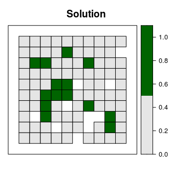
This solution is even better then the previous solution. However, we are not finished yet. This solution does not maintain connectivity between reserves, and so species may have limited capacity to disperse throughout the solution. To avoid this, we can add contiguity constraints (add_contiguity_constraints).
# create new problem with contiguity constraints
p4 <- p3 %>%
      add_contiguity_constraints()

# solve the problem
s4 <- solve(p4)
## Gurobi Optimizer version 9.0.2 build v9.0.2rc0 (linux64)
## Optimize a model with 654 rows, 506 columns and 2292 nonzeros
## Model fingerprint: 0x1ced3129
## Variable types: 0 continuous, 506 integer (506 binary)
## Coefficient statistics:
## Matrix range [2e-01, 1e+00]
## Objective range [6e+01, 3e+02]
## Bounds range [1e+00, 1e+00]
## RHS range [1e+00, 1e+01]
## Presolve removed 340 rows and 252 columns
## Presolve time: 0.01s
## Presolved: 314 rows, 254 columns, 702 nonzeros
## Variable types: 0 continuous, 254 integer (254 binary)
## Found heuristic solution: objective 7270.1195351
## Found heuristic solution: objective 6070.2074533
## Presolved: 314 rows, 254 columns, 702 nonzeros
##
##
## Root relaxation: objective 5.489159e+03, 69 iterations, 0.00 seconds
##
## Nodes | Current Node | Objective Bounds | Work
## Expl Unexpl | Obj Depth IntInf | Incumbent BestBd Gap | It/Node Time
##
## 0 0 5489.15943 0 59 6070.20745 5489.15943 9.57% - 0s
## H 0 0 5859.8468810 5489.15943 6.33% - 0s
## H 0 0 5858.4184908 5489.15943 6.30% - 0s
## 0 0 5738.84421 0 49 5858.41849 5738.84421 2.04% - 0s
## 0 0 5738.84421 0 29 5858.41849 5738.84421 2.04% - 0s
## 0 0 5814.59442 0 22 5858.41849 5814.59442 0.75% - 0s
## 0 0 cutoff 0 5858.41849 5858.41849 0.00% - 0s
##
## Cutting planes:
## Gomory: 6
## Zero half: 8
## RLT: 6
##
## Explored 1 nodes (241 simplex iterations) in 0.03 seconds
## Thread count was 1 (of 4 available processors)
##
## Solution count 4: 5858.42 5859.85 6070.21 7270.12
##
## Optimal solution found (tolerance 0.00e+00)
## Best objective 5.858418490821e+03, best bound 5.858418490821e+03, gap 0.0000%# plot the solution
spplot(s4, "solution_1", main = "Solution", at = c(0, 0.5, 1.1),
col.regions = c("grey90", "darkgreen"), xlim = c(-0.1, 1.1),
ylim = c(-0.1, 1.1))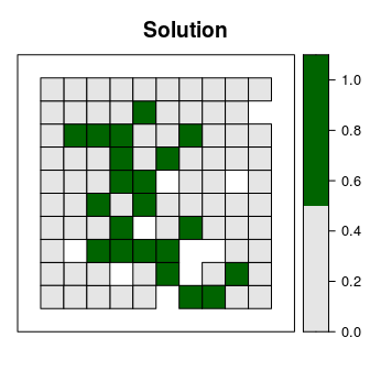
Now let’s explore which planning units selected in the prioritization are most important for meeting our targets as cost-effectively as possible. To achieve this, we will calculate irreplaceability scores using the replacement cost method. Under this method, planning units with higher scores are more irreplaceable than those with lower scores. Furthermore, planning units with infinite scores are critical—it is impossible to meet our targets without protecting these planning units. Note that we override the solver behavior in the code below to prevent lots of unnecessary text from being output.
# solve the problem
rc <- p4 %>%
      add_default_solver(gap = 0, verbose = FALSE) %>%
      replacement_cost(s4[, "solution_1"])
## Warning in res(x, ...): overwriting previously defined solver# set infinite values as 1.09 so we can plot them
rc$rc[rc$rc > 100] <- 1.09
# plot the irreplaceability scores
# planning units that are replaceable are shown in purple, blue, green, and
# yellow, and planning units that are truly irreplaceable are shown in red
spplot(rc, "rc", main = "Irreplaceability", xlim = c(-0.1, 1.1),
ylim = c(-0.1, 1.1), at = c(seq(0, 0.9, 0.1), 1.01, 1.1),
col.regions = c("#440154", "#482878", "#3E4A89", "#31688E", "#26828E",
"#1F9E89", "#35B779", "#6DCD59", "#B4DE2C", "#FDE725",
"#FF0000"))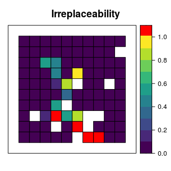
This short example demonstrates how the prioritizr R package can be used to build a minimal conservation problem, how constraints and penalties can be iteratively added to the problem to obtain a solution, and how irreplaceability scores can be calculated for the solution to identify critical places. Although we explored just a few different functions for modifying the a conservation problem, the prioritizr R package provides many functions for specifying objectives, constraints, penalties, and decision variables, so that you can build and custom-tailor a conservation planning problem to suit your exact planning scenario.
Please refer to the package website for more information on the prioritizr R package. This website contains a comprehensive tutorial on the package, instructions for installing the Gurobi software suite to solve large-scale and complex conservation planning problems, and a tutorial on solving problems with multiple management zones. It also provides two worked examples that involve real-world data from Tasmania, Australia and Salt Spring Island, Canada. Additionally, slides for previous seminars about the package can be found in teaching repository. Furthermore, materials accompanying previous workshops are also available online too (i.e. the CIBIO 2019 workshop and the PacMara 2019 workshop). If you have any questions about using the prioritizr R package or suggestions for improving it, please file an issue at the package’s online code repository.