pre is an R package for deriving prediction rule ensembles for binary, multinomial, (multivariate) continuous, count and survival responses. Input variables may be numeric, ordinal and categorical. An extensive description of the implementation and functionality is provided in Fokkema (2017). The package largely implements the algorithm for deriving prediction rule ensembles as described in Friedman & Popescu (2008), with several adjustments:
gpe().Note that pre is under development, and much work still needs to be done. Below, a short introductory example is provided. Fokkema (2017) provides an extensive description of the fitting procedures implemented in function pre() and example analyses with more extensive explanations.
To get a first impression of how function pre() works, we will fit a prediction rule ensemble to predict Ozone levels using the airquality dataset. We fit a prediction rule ensemble using function pre():
library("pre")
airq <- airquality[complete.cases(airquality), ]
set.seed(42)
airq.ens <- pre(Ozone ~ ., data = airq)
Note that it is necessary to set the random seed, to allow for later replication of the results, because the fitting procedure depends on random sampling of training observations.
We can print the resulting ensemble (alternatively, we could use the print method):
airq.ens
#>
#> Final ensemble with cv error within 1se of minimum:
#>   lambda =  3.543968
#>   number of terms = 12
#>   mean cv error (se) = 352.3834 (99.13981)
#>
#>   cv error type : Mean-Squared Error
#>
#>          rule   coefficient                          description
#>   (Intercept)   68.48270406                                    1
#>       rule191  -10.97368179              Wind > 5.7 & Temp <= 87
#>       rule173  -10.90385520              Wind > 5.7 & Temp <= 82
#>        rule42   -8.79715538              Wind > 6.3 & Temp <= 84
#>       rule204    7.16114780         Wind <= 10.3 & Solar.R > 148
#>        rule10   -4.68646144              Temp <= 84 & Temp <= 77
#>       rule192   -3.34460037  Wind > 5.7 & Temp <= 87 & Day <= 23
#>        rule51   -2.27864287              Wind > 5.7 & Temp <= 84
#>        rule93    2.18465676              Temp > 77 & Wind <= 8.6
#>        rule74   -1.36479546              Wind > 6.9 & Temp <= 84
#>        rule28   -1.15326093              Temp <= 84 & Wind > 7.4
#>        rule25   -0.70818399              Wind > 6.3 & Temp <= 82
#>       rule166   -0.04751152              Wind > 6.9 & Temp <= 82
The firest few lines of the printed results provide the penalty parameter value (λ) employed for selecting the final ensemble. By default, the ‘1-SE’ rule is used for selecting λ; this default can be overridden by employing the penalty.par.val argument of the print method and other functions in the package. Note that the printed cross-validated error is calculated using the same data as was used for generating the rules and likely provides an overly optimistic estimate of future prediction error. To obtain a more realistic prediction error estimate, we will use function cvpre() later on.
Next, the printed results provide the rules and linear terms selected in the final ensemble, with their estimated coefficients. For rules, the description column provides the conditions. For linear terms (which were not selected in the current ensemble), the winsorizing points used to reduce the influence of outliers on the estimated coefficient would be printed in the description column. The coefficient column presents the estimated coefficient. These are regression coefficients, reflecting the expected increase in the response for a unit increase in the predictor, keeping all other predictors constant. For rules, the coefficient thus reflects the difference in the expected value of the response when the conditions of the rule are met, compared to when they are not.
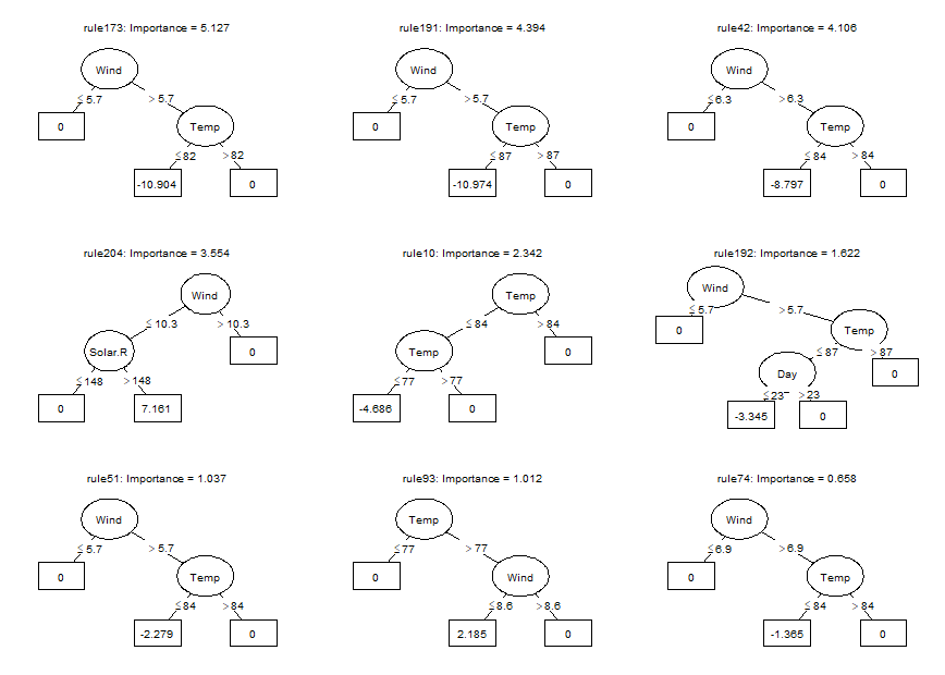
Using the plot method, we can plot the rules in the ensemble as simple decision trees. Here, we will request the nine most important baselearners through specification of the nterms argument. Through the cex argument, we specify the size of the node and path labels:
Using the coef method, we can obtain the estimated coefficients for each of the baselearners (we only print the first six terms here for space considerations):
coefs <- coef(airq.ens)
coefs[1:6, ]
#>            rule coefficient                  description
#> 201 (Intercept)   68.482704                            1
#> 167     rule191  -10.973682      Wind > 5.7 & Temp <= 87
#> 150     rule173  -10.903855      Wind > 5.7 & Temp <= 82
#> 39       rule42   -8.797155      Wind > 6.3 & Temp <= 84
#> 179     rule204    7.161148 Wind <= 10.3 & Solar.R > 148
#> 10       rule10   -4.686461      Temp <= 84 & Temp <= 77
We can generate predictions for new observations using the predict method (only the first six predicted values are printed here for space considerations):
predict(airq.ens, newdata = airq[1:6, ])
#>        1        2        3        4        7        8
#> 32.53896 24.22456 24.22456 24.22456 31.38570 24.22456
Using function cvpre(), we can assess the expected prediction error of the fitted PRE through k-fold cross validation (k = 10, by default, which can be overridden through specification of the k argument):
set.seed(43)
airq.cv <- cvpre(airq.ens)
#> $MSE
#>      MSE       se
#> 369.2010  88.7574
#>
#> $MAE
#>      MAE       se
#> 13.64524  1.28985
The results provide the mean squared error (MSE) and mean absolute error (MAE) with their respective standard errors. These results are saved for later use in aiq.cv$accuracy. The cross-validated predictions, which can be used to compute alternative estimates of predictive accuracy, are saved in airq.cv$cvpreds. The folds to which observations were assigned are saved in airq.cv$fold_indicators.
Package pre provides several additional tools for interpretation of the final ensemble. These may be especially helpful for complex ensembles containing many rules and linear terms.
We can assess the relative importance of input variables as well as baselearners using the importance() function:
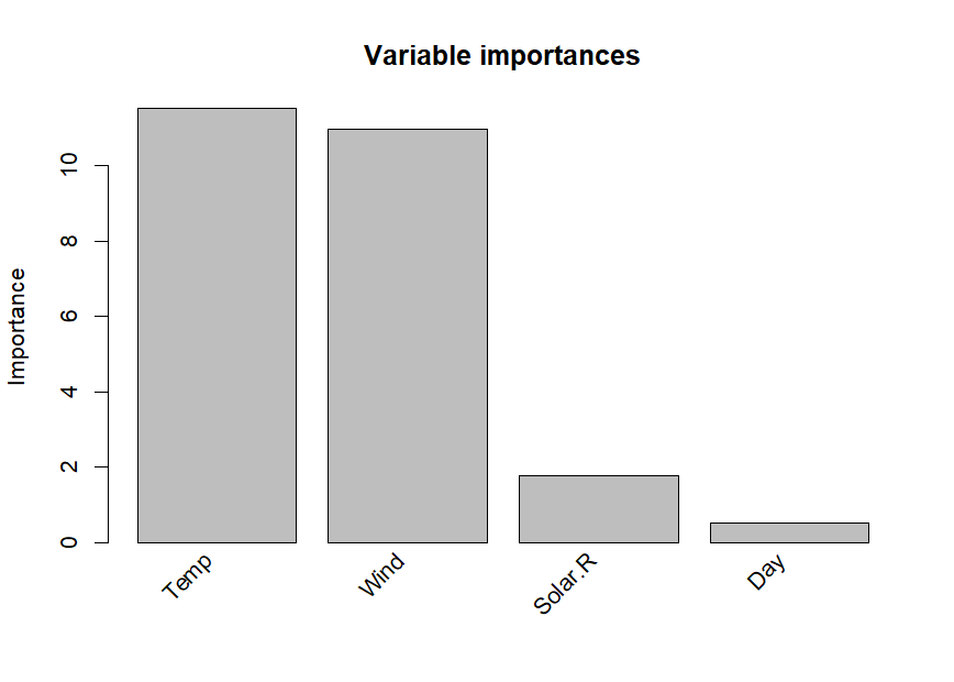
As we already observed in the printed ensemble, the plotted variable importances indicate that Temperature and Wind are most strongly associated with Ozone levels. Solar.R and Day are also associated with Ozone levels, but much less strongly. Variable Month is not plotted, which means it obtained an importance of zero, indicating that it is not associated with Ozone levels. We already observed this in the printed ensemble: Month did not appear in any of the selected terms. The variable and baselearner importances are saved for later use in imps$varimps and imps$baseimps, respectively.
We can obtain explanations of the predictions for individual observations using function explain():
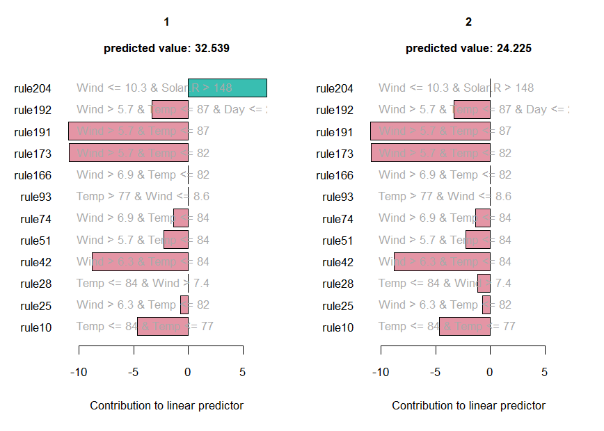
The values of the rules and linear terms for each observation are saved in expl$predictors, their contributions in expl$contribution and the predicted values in expl$predicted.value.
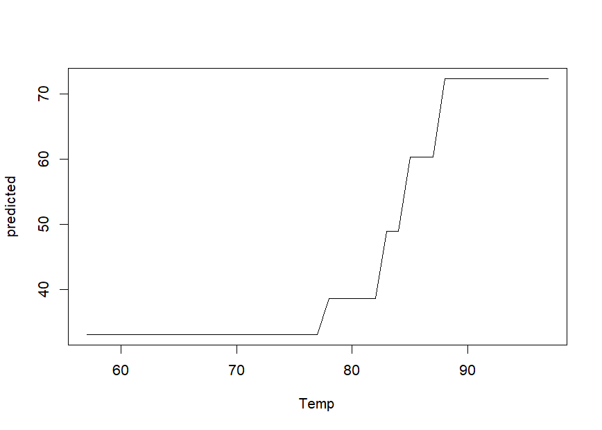
We can obtain partial dependence plots to assess the effect of single predictor variables on the outcome using the singleplot() function:
We can obtain partial dependence plots to assess the effects of pairs of predictor variables on the outcome using the pairplot() function:
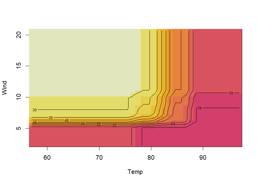
Note that creating partial dependence plots is computationally intensive and computation time will increase fast with increasing numbers of observations and numbers of variables. **R** package **plotmo** (Milborrow (2018)) provides more efficient functions for plotting partial dependence, which also support pre models.
If the final ensemble does not contain many terms, inspecting individual rules and linear terms through the print method may be more informative than partial dependence plots. One of the main advantages of prediction rule ensembles is their interpretability: the predictive model contains only simple functions of the predictor variables (rules and linear terms), which are easy to grasp. Partial dependence plots are often much more useful for interpretation of complex models, like random forests for example.
We can assess the presence of interactions between the input variables using the interact() and bsnullinteract() funtions. Function bsnullinteract() computes null-interaction models (10, by default) based on bootstrap-sampled and permuted datasets. Function interact() computes interaction test statistics for each predictor variables appearing in the specified ensemble. If null-interaction models are provided through the nullmods argument, interaction test statistics will also be computed for the null-interaction model, providing a reference null distribution.
Note that computing null interaction models and interaction test statistics is computationally very intensive, so running the following code will take some time:
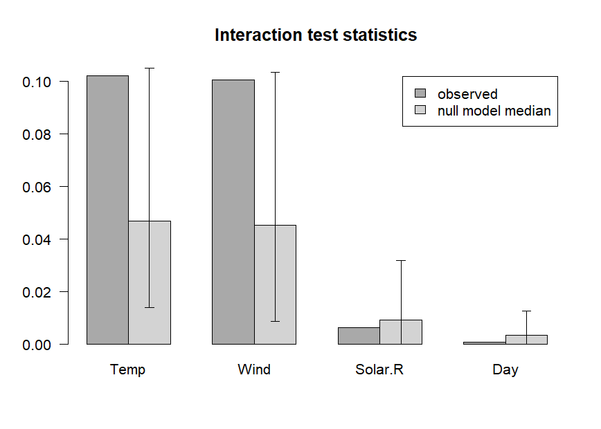
The plotted variable interaction strengths indicate that Temperature and Wind may be involved in interactions, as their observed interaction strengths (darker grey) exceed the upper limit of the 90% confidence interval (CI) of interaction stengths in the null interaction models (lighter grey bar represents the median, error bars represent the 90% CIs). The plot indicates that Solar.R and Day are not involved in any interactions. Note that computation of null interaction models is computationally intensive. A more reliable result can be obtained by computing a larger number of boostrapped null interaction datasets, by setting the nsamp argument of function bsnullinteract() to a larger value (e.g., 100).
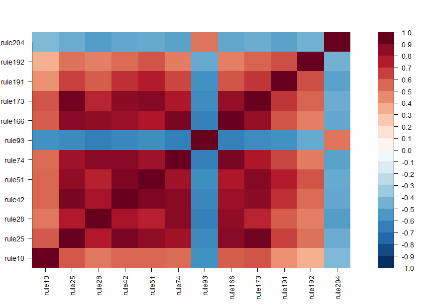
We can assess correlations between the baselearners appearing in the ensemble using the corplot() function:
More complex prediction ensembles can be obtained using the gpe() function. Abbreviation gpe stands for generalized prediction ensembles, which can also include hinge functions of the predictor variables as described in Friedman (1991), in addition to rules and/or linear terms. Addition of hinge functions may further improve predictive accuracy. See the following example:
set.seed(42)
airq.gpe <- gpe(Ozone ~ ., data = airquality[complete.cases(airquality),],
    base_learners = list(gpe_trees(), gpe_linear(), gpe_earth()))
airq.gpe
#>
#> Final ensemble with cv error within 1se of minimum:
#>   lambda =  3.229132
#>   number of terms = 11
#>   mean cv error (se) = 361.2152 (110.9785)
#>
#>   cv error type : Mean-squared Error
#>
#>                                   description  coefficient
#>                                   (Intercept)  65.52169487
#>                                    Temp <= 77  -6.20973854
#>                  Wind <= 10.3 & Solar.R > 148   5.46410965
#>                       Wind > 5.7 & Temp <= 82  -8.06127416
#>                       Wind > 5.7 & Temp <= 84  -7.16921733
#>                       Wind > 5.7 & Temp <= 87  -8.04255470
#>           Wind > 5.7 & Temp <= 87 & Day <= 23  -3.40525575
#>                       Wind > 6.3 & Temp <= 82  -2.71925536
#>                       Wind > 6.3 & Temp <= 84  -5.99085126
#>                       Wind > 6.9 & Temp <= 82  -0.04406376
#>                       Wind > 6.9 & Temp <= 84  -0.55827336
#>   eTerm(Solar.R * h(9.7 - Wind), scale = 410)   9.91783318
#>
#> 'h' in the 'eTerm' indicates the hinge functionBreiman, L., Friedman, J., Olshen, R., & Stone, C. (1984). Classification and regression trees. Boca Raton, FL: Chapman&Hall/CRC.
Fokkema, M. (2017). pre: An R package for fitting prediction rule ensembles. arXiv:1707.07149. Retrieved from https://arxiv.org/abs/1707.07149
Friedman, J. (1991). Multivariate adaptive regression splines. The Annals of Statistics, 19(1), 1–67.
Friedman, J., & Popescu, B. (2008). Predictive learning via rule ensembles. The Annals of Applied Statistics, 2(3), 916–954. Retrieved from http://www.jstor.org/stable/30245114
Hothorn, T., Hornik, K., & Zeileis, A. (2006). Unbiased recursive partitioning: A conditional inference framework. Journal of Computational and Graphical Statistics, 15(3), 651–674.
Milborrow, S. (2018). plotmo: Plot a model’s residuals, response, and partial dependence plots. Retrieved from https://CRAN.R-project.org/package=plotmo
Zeileis, A., Hothorn, T., & Hornik, K. (2008). Model-based recursive partitioning. Journal of Computational and Graphical Statistics, 17(2), 492–514.