Describe and understand your model’s parameters!
parameters’ primary goal is to provide utilities for processing the parameters of various statistical models (see here for a list of supported models). Beyond computing p-values, CIs, Bayesian indices and other measures for a wide variety of models, this package implements features like bootstrapping of parameters and models, feature reduction (feature extraction and variable selection).
Run the following:
![]()
![]()
![]()
Click on the buttons above to access the package documentation and the easystats blog, and check-out these vignettes:
In case you want to file an issue or contribute in another way to the package, please follow this guide. For questions about the functionality, you may either contact us via email or also file an issue.
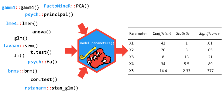
The model_parameters() function (that can be accessed via the parameters() shortcut) allows you to extract the parameters and their characteristics from various models in a consistent way. It can be considered as a lightweight alternative to broom::tidy(), with some notable differences:
standardize_names()).model <- lm(Sepal.Width ~ Petal.Length * Species + Petal.Width, data = iris)
# regular model parameters
model_parameters(model)
#> Parameter | Coefficient | SE | 95% CI | t | df | p
#> ------------------------------------------------------------------------------------------------
#> (Intercept) | 2.89 | 0.36 | [ 2.18, 3.60] | 8.01 | 143 | < .001
#> Petal.Length | 0.26 | 0.25 | [-0.22, 0.75] | 1.07 | 143 | 0.287
#> Species [versicolor] | -1.66 | 0.53 | [-2.71, -0.62] | -3.14 | 143 | 0.002
#> Species [virginica] | -1.92 | 0.59 | [-3.08, -0.76] | -3.28 | 143 | 0.001
#> Petal.Width | 0.62 | 0.14 | [ 0.34, 0.89] | 4.41 | 143 | < .001
#> Petal.Length * Species [versicolor] | -0.09 | 0.26 | [-0.61, 0.42] | -0.36 | 143 | 0.721
#> Petal.Length * Species [virginica] | -0.13 | 0.26 | [-0.64, 0.38] | -0.50 | 143 | 0.618
# standardized parameters
model_parameters(model, standardize = "refit")
#> Parameter | Coefficient | SE | 95% CI | t | df | p
#> ------------------------------------------------------------------------------------------------
#> (Intercept) | 3.59 | 1.30 | [ 1.01, 6.17] | 2.75 | 143 | 0.007
#> Petal.Length | 1.07 | 1.00 | [-0.91, 3.04] | 1.07 | 143 | 0.287
#> Species [versicolor] | -4.62 | 1.31 | [-7.21, -2.03] | -3.53 | 143 | < .001
#> Species [virginica] | -5.51 | 1.38 | [-8.23, -2.79] | -4.00 | 143 | < .001
#> Petal.Width | 1.08 | 0.24 | [ 0.59, 1.56] | 4.41 | 143 | < .001
#> Petal.Length * Species [versicolor] | -0.38 | 1.06 | [-2.48, 1.72] | -0.36 | 143 | 0.721
#> Petal.Length * Species [virginica] | -0.52 | 1.04 | [-2.58, 1.54] | -0.50 | 143 | 0.618library(lme4)
model <- lmer(Sepal.Width ~ Petal.Length + (1|Species), data = iris)
# model parameters with CI, df and p-values based on Wald approximation
model_parameters(model)
#> Parameter | Coefficient | SE | 95% CI | t | df | p
#> ----------------------------------------------------------------------
#> (Intercept) | 2.00 | 0.56 | [0.90, 3.10] | 3.56 | 146 | < .001
#> Petal.Length | 0.28 | 0.06 | [0.17, 0.40] | 4.75 | 146 | < .001
# model parameters with CI, df and p-values based on Kenward-Roger approximation
model_parameters(model, df_method = "kenward")
#> Parameter | Coefficient | SE | 95% CI | t | df | p
#> -------------------------------------------------------------------------
#> (Intercept) | 2.00 | 0.57 | [0.07, 3.93] | 3.53 | 2.67 | 0.046
#> Petal.Length | 0.28 | 0.06 | [0.16, 0.40] | 4.58 | 140.98 | < .001Besides many types of regression models and packages, it also works for other types of models, such as structural models (EFA, CFA, SEM…).
library(psych)

model <- psych::fa(attitude, nfactors = 3)
model_parameters(model)
#> # Rotated loadings from Factor Analysis (oblimin-rotation)
#>
#> Variable   |   MR1 |   MR2 |   MR3 | Complexity | Uniqueness
#> ------------------------------------------------------------
#> rating     |  0.90 | -0.07 | -0.05 |       1.02 |       0.23
#> complaints |  0.97 | -0.06 |  0.04 |       1.01 |       0.10
#> privileges |  0.44 |  0.25 | -0.05 |       1.64 |       0.65
#> learning   |  0.47 |  0.54 | -0.28 |       2.51 |       0.24
#> raises     |  0.55 |  0.43 |  0.25 |       2.35 |       0.23
#> critical   |  0.16 |  0.17 |  0.48 |       1.46 |       0.67
#> advance    | -0.11 |  0.91 |  0.07 |       1.04 |       0.22
#>
#> The 3 latent factors (oblimin rotation) accounted for 66.60% of the total variance of the original data (MR1 = 38.19%, MR2 = 22.69%, MR3 = 5.72%).
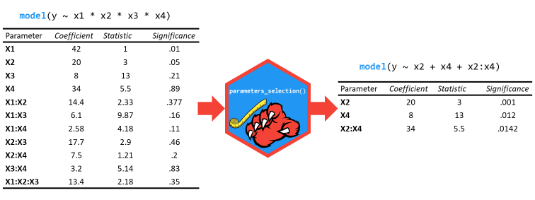
select_parameters() can help you quickly select and retain the most relevant predictors using methods tailored for the model type.
library(dplyr)

lm(disp ~ ., data = mtcars) %>%
  select_parameters() %>%
  model_parameters()
#> Parameter   | Coefficient |     SE |            95% CI |     t | df |      p
#> ----------------------------------------------------------------------------
#> (Intercept) |      141.70 | 125.67 | [-116.62, 400.02] |  1.13 | 26 | 0.270
#> cyl         |       13.14 |   7.90 | [  -3.10,  29.38] |  1.66 | 26 | 0.108
#> hp          |        0.63 |   0.20 | [   0.22,   1.03] |  3.18 | 26 | 0.004
#> wt          |       80.45 |  12.22 | [  55.33, 105.57] |  6.58 | 26 | < .001
#> qsec        |      -14.68 |   6.14 | [ -27.31,  -2.05] | -2.39 | 26 | 0.024
#> carb | -28.75 | 5.60 | [ -40.28, -17.23] | -5.13 | 26 | < .001This packages also contains a lot of other useful functions:
data(iris)
describe_distribution(iris)
#> Variable     | Mean |   SD |  IQR |        Range | Skewness | Kurtosis |   n | n_Missing
#> ----------------------------------------------------------------------------------------
#> Sepal.Length | 5.84 | 0.83 | 1.30 | [4.30, 7.90] |     0.31 |    -0.55 | 150 |         0
#> Sepal.Width  | 3.06 | 0.44 | 0.52 | [2.00, 4.40] |     0.32 |     0.23 | 150 |         0
#> Petal.Length | 3.76 | 1.77 | 3.52 | [1.00, 6.90] |    -0.27 |    -1.40 | 150 |         0
#> Petal.Width | 1.20 | 0.76 | 1.50 | [0.10, 2.50] | -0.10 | -1.34 | 150 | 0In order to cite this package, please use the following citation:
Corresponding BibTeX entry:
@Article{,
  title = {Describe and understand your model's parameters},
  author = {Daniel Lüdecke and Mattan S. Ben-Shachar and Dominique Makowski},
  journal = {CRAN},
  year = {2019},
  note = {R package},
  url = {https://github.com/easystats/parameters},
}