![]() ## packageRank: compute and visualize package download counts and rank percentiles
## packageRank: compute and visualize package download counts and rank percentiles
‘packageRank’ is an R package that helps put package download counts into context. It does so via two functions, cranDownloads() and packageRank(). cranDownloads() extends cranlogs::cran_downloads() package by adding a plot() method and a more user-friendly interface to the task of counting package downloads. packageRank() uses rank percentiles, a nonparametric statistic that tells you the percentage of packages with fewer downloads, to help you see how your package is doing compared to all other packages on CRAN.
NOTE: ‘packageRank’relies on the ‘cranlogs’ package and requires an active internet connection. ‘cranlogs’ uses the RStudio logs to compute package downloads. These logs record traffic to what was previously RStudio’s CRAN mirror (cran.rstudio.com) and is currently the “0-Cloud” mirror (cloud.r-project.org), which is “sponsored by RStudio”. Note that the logs for the previous day are generally posted the next day at 18:00 (GMT+1) or 17:00 UTC (GMT+2) (daylight saving time); results for functions that rely on ‘cranlogs’ are available soon after.
To install ‘packageRank’ from CRAN:
To install the development version from GitHub:
# You may need to first install 'remotes' via install.packages("remotes").
remotes::install_github("lindbrook/packageRank", build_vignettes = TRUE)cranDownloads() uses all the same arguments as cranlogs::cran_downloads():
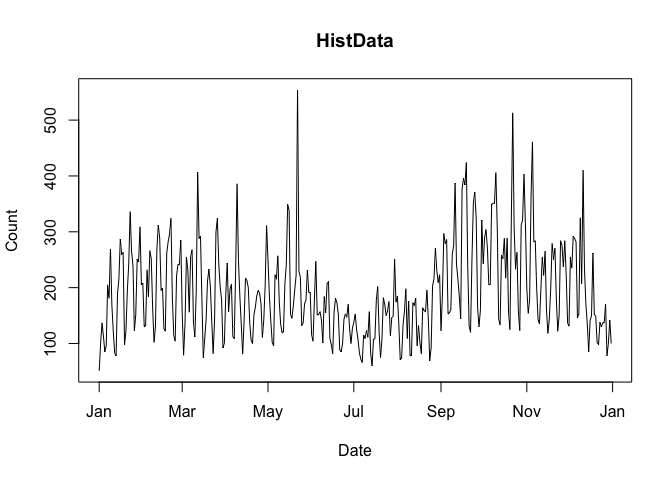
>         date count  package
> 1 2020-05-01 338 HistData> date count package
> 1 2020-05-01 338 HistDataThe only difference is that cranDownloads() adds three features:
## Error in cranDownloads(packages = "GGplot2") :
## GGplot2: misspelled or not on CRAN.> date count package
> 1 2020-05-01 56357 ggplot2
This also works for inactive or “retired” packages in the Archive:
## Error in cranDownloads(packages = "vr") :
## vr: misspelled or not on CRAN/Archive.> date count package
> 1 2020-05-01 11 VRWith cranlogs::cran_downloads(), you specify a time frame using the from and to arguments. The downside of this is that dates must use the “yyyy-mm-dd” format. For convenience’s sake and to reduce typing, cranDownloads() also allows you to use “yyyy-mm” or “yyyy” (yyyy also works).
Let’s say you want the download counts for ‘HistData’ from February 2020. With cranlogs::cran_downloads(), you have to type out the whole date and remember that 2020 was a leap year:
With cranDownloads(), you can just specify the year and month:
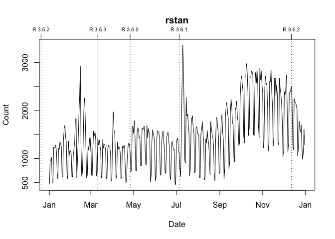
Let’s say you want the year-to-date download counts for ‘rstan’. With cranlogs::cran_downloads(), you’d type something like:
With cranDownloads(), you can just type:
cranDownloads() tries to check for valid dates:
## Error in resolveDate(to, type = "to") : Not a valid date.cranDownloads() makes visualization easy. Just use plot():
If you pass a vector of package names for a single day, plot() returns a dotchart:
plot(cranDownloads(packages = c("ggplot2", "data.table", "Rcpp"),
  from = "2020-03-01", to = "2020-03-01"))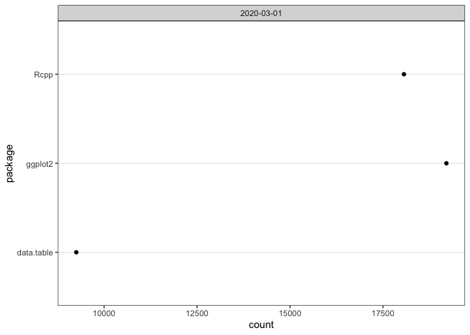
If you pass a vector of package names, plot() will use ggplot2 facets:
plot(cranDownloads(packages = c("ggplot2", "data.table", "Rcpp"),
  from = "2020", to = "2020-03-20"))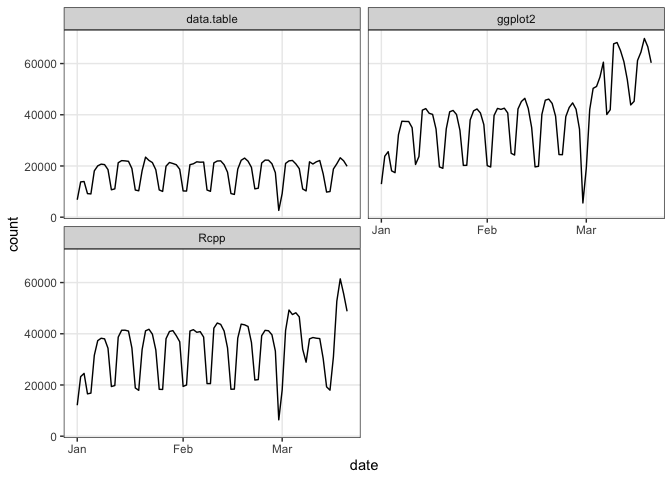
If you want to plot those data in a single frame, use multi.plot = TRUE:
plot(cranDownloads(packages = c("ggplot2", "data.table", "Rcpp"),
  from = "2020", to = "2020-03-20"), multi.plot = TRUE)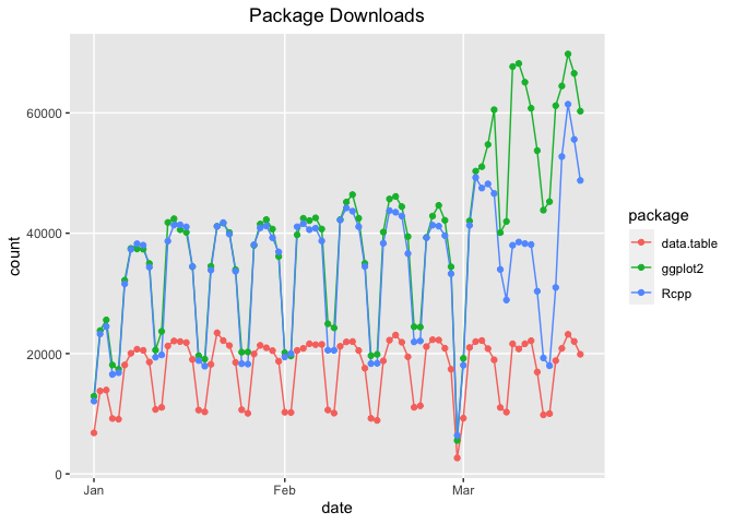
If you want separate plots, use graphics = "base" (you’ll be prompted for each plot):
plot(cranDownloads(packages = c("ggplot2", "data.table", "Rcpp"),
  from = "2020", to = "2020-03-20"), graphics = "base")
If you want separate, independently scaled plots, add same.xy = FALSE:
plot(cranDownloads(packages = c("ggplot2", "data.table", "Rcpp"),
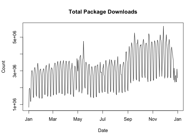
from = "2020", to = "2020-03-20"), graphics = "base", same.xy = FALSE)packages = NULLcranlogs::cran_download(packages = NULL) computes the total number of package downloads from CRAN.
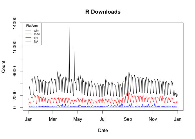
packages = "R"cranlogs::cran_download(packages = "R") computes the total number of downloads of the R application (note that you can only use “R” or a vector of packages names, not both!).
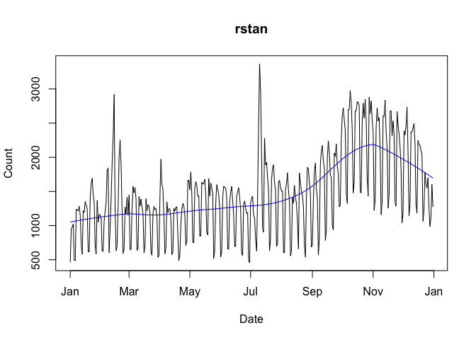
To add a lowess smoother to your data, use smooth = TRUE:
With graphs that use ‘ggplot2’, se = TRUE will add confidence intervals:
plot(cranDownloads(packages = c("HistData", "rnaturalearth", "Zelig"),
  from = "2020", to = "2020-03-20"), smooth = TRUE, se = TRUE)
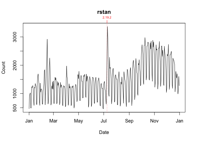
To annotate a graph with package release dates:
To annotate a graph with R release dates:
To visualize a package’s downloads relative to “all” other packages over time:
plot(cranDownloads(packages = "HistData", from = "2020", to = "2020-03-20"),
  population.plot = TRUE)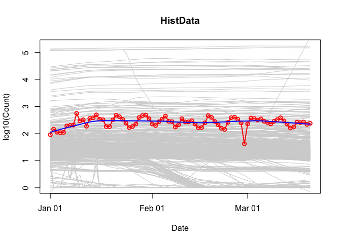
This longitudinal view plots the date (x-axis) against the logarithm of a package’s downloads (y-axis). In the background, the same variable are plotted (in gray) for a stratified random sample of packages: within each 5% interval of rank percentiles (e.g., 0 to 5, 5 to 10, 95 to 100, etc.), a random sample of 5% of packages is selected and tracked over time. This sample approximates the “typical” pattern of downloads for that time period.
After looking the download count data for a while, the “compared to what?” question will quickly come to mind. For instance, consider the data for the first week of March 2020:
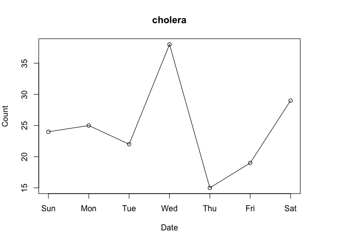
Do Wednesday and Saturday reflect surges of interest in the package or surges of traffic to CRAN? To put it differently, how can we know if a given download count is typical or unusual?
One way to answer these questions is to locate your package in the frequency distribution of download counts. Below are the distributions for Wednesday and Saturday with the location of ‘cholera’ highlighted:
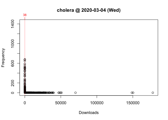
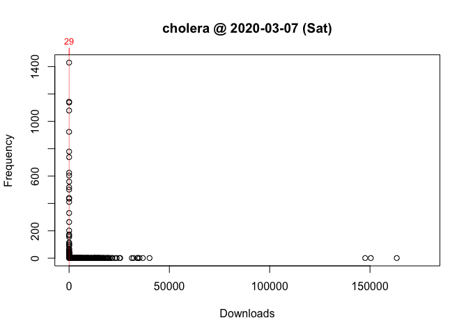
As you can see, the frequency distribution of package downloads typically has a heavily skewed, exponential shape. On the Wednesday, the most “popular” package had 177,745 downloads while the least “popular” package(s) had just one. This is why the left side of the distribution, where packages with fewer downloads are located, looks like a vertical line.
To see what’s going on, I take the log of download counts (x-axis) and redraw the graph. In these plots, the location of a vertical segment along the x-axis represents a download count and the height of a vertical segment represents the frequency of a download count:
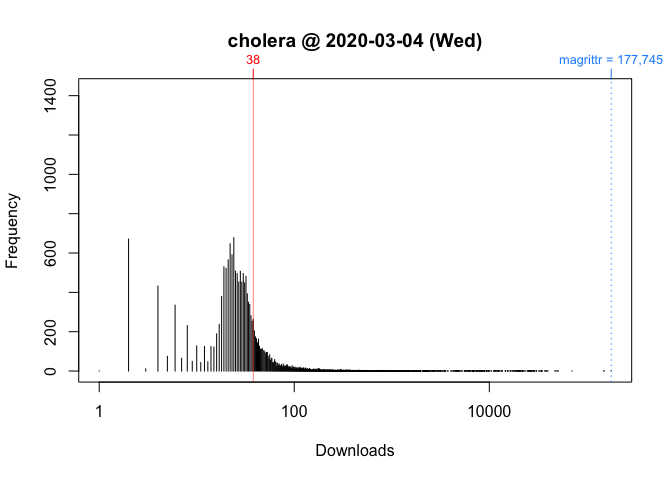
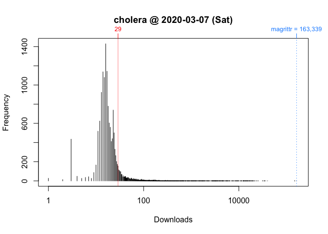
While these plots give us a better picture of where ‘cholera’ is located, comparisons between Wednesday and Saturday are impressionistic at best: all we can confidently say is that the download counts for both days were greater than the mode.
To facilitate interpretation and comparison, I use the rank percentile of download counts in place of nominal download counts. This nonparametric statistic tells you the percentage of packages with fewer downloads. In other words, it gives you the location of your package relative to the locations of all other packages. More importantly, by rescaling download counts to lie on the bounded interval between 0 and 100, rank percentiles make it easier to compare packages within and across distributions.
For example, we can compare Wednesday (“2020-03-04”) to Saturday (“2020-03-07”):
packageRank(package = "cholera", date = "2020-03-04", size.filter = FALSE)
>         date packages downloads            rank percentile
> 1 2020-03-04  cholera        38 5,556 of 18,038       67.9
On Wednesday, we can see that ‘cholera’ had 38 downloads, came in 5,556th place out of 18,038 unique packages downloaded, and earned a spot in the 68th percentile.
packageRank(package = "cholera", date = "2020-03-07", size.filter = FALSE)
>         date packages downloads            rank percentile
> 1 2020-03-07  cholera        29 3,061 of 15,950         80
On Saturday, we can see that ‘cholera’ had 29 downloads, came in 3,061st place out of 15,950 unique packages downloaded, earned a spot in the 80th percentile.
So contrary to what the nominal counts tell us, one could say that the interest in ‘cholera’ was actually greater on Saturday than on Wednesday.
To compute rank percentiles, I do the following. For each package, I tabulate the number of downloads and then compute the percentage of packages with fewer downloads. Here are the details using ‘cholera’ from Wednesday as an example:
pkg.rank <- packageRank(packages = "cholera", date = "2020-03-04",
  size.filter = FALSE)

downloads <- pkg.rank$crosstab

round(100 * mean(downloads < downloads["cholera"]), 1)
> [1] 67.9
To put it differently:
(pkgs.with.fewer.downloads <- sum(downloads < downloads["cholera"]))
> [1] 12250

(tot.pkgs <- length(downloads))
> [1] 18038

round(100 * pkgs.with.fewer.downloads / tot.pkgs, 1)
> [1] 67.9
For the example above, 38 downloads puts ‘HistData’ in 5,556th place among the 18,038 packages downloaded.
This rank is “nominal” because multiple packages can have the same number of downloads. As a result, a package’s nominal rank (but not its rank percentile) can be affected by its name: packages with the same number of downloads are sorted in alphabetical order.
Thus, ‘HistData’ benefits from the fact that it is 31st in the list of 263 packages with 38 downloads:
pkg.rank <- packageRank(packages = "cholera", date = "2020-03-04",
  size.filter = FALSE)
downloads <- pkg.rank$crosstab

which(names(downloads[downloads == 38]) == "cholera")
> [1] 31
length(downloads[downloads == 38])
> [1] 263To visualize packageRank(), use plot().
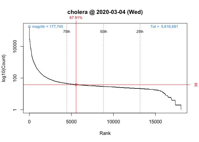
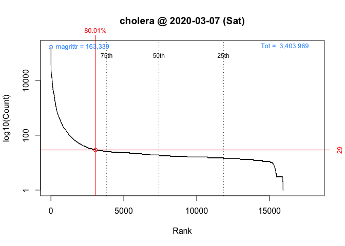
These graphs, customized to be on the same scale, plot the rank order of packages’ download counts (x-axis) against the logarithm of those counts (y-axis). It then highlights a package’s position in the distribution along with its rank percentile and download count (in red). In the background, the 75th, 50th and 25th percentiles are plotted as dotted vertical lines; the package with the most downloads, which in both cases is ‘magrittr’ (in blue, top left); and the total number of downloads, 5,561,681 and 3,403,969 respectively (in blue, top right).
packageRank() and packageLog() have an additional argument, ‘size.filter’ that by removes downloads < 1000 bytes. Depending on the day of the week and the number of versions a package has, this can provide a more accurate count of package downloads. For example, here is a raw download count:
packageRank(packages = "HistData", date = "2019-10-30", size.filter = FALSE)
>         date packages downloads          rank percentile
> 1 2019-10-30 HistData       403 794 of 17,396       95.4
Below is a filtered count.
packageRank(packages = "HistData", date = "2019-10-30", size.filter = TRUE)
>         date packages downloads          rank percentile
> 1 2019-10-30 HistData       382 796 of 15,330       94.8
Besides a difference of 21 downloads, notice that the number of unique packages downloaded falls from 17,396 to 15,330.
By default, size.filter = TRUE for packageRank() and size.filter = FALSE for packageLog().
To avoid the bottleneck of downloading multiple log files, packageRank() is currently limited to individual days or observations. However, to reduce the need to re-download logs, ‘packageRank’ makes use of memoization via the ‘memoise’ package.
Here’s relevant code:
fetchLog <- function(url) data.table::fread(url)

mfetchLog <- memoise::memoise(fetchLog)

if (RCurl::url.exists(url)) {
  cran_log <- mfetchLog(url)
}

# Note that data.table::fread() relies on R.utils::decompressFile().
If you use fetchLog(), the log file, which can be upwards of 50 MB, will be downloaded every time you call the function. If you use mfetchLog(), logs are intelligently cached; those that have already been downloaded, in your current R session, will not be downloaded again.