modelbased

modelbased is a lightweight package helping with model-based estimations, used in the computation of marginal means, contrast analysis and predictions.

Installation

Run the following:

install.packages("devtools")
devtools::install_github("easystats/modelbased")

library("modelbased")

Documentation

Click on the buttons above to access the package documentation and the easystats blog, and check-out these vignettes:

• Visualisation matrix
• Marginal means
• Contrast analysis
• Use a model to make predictions
• Describe non-linear curves

Features

The package is built around 5 main functions:

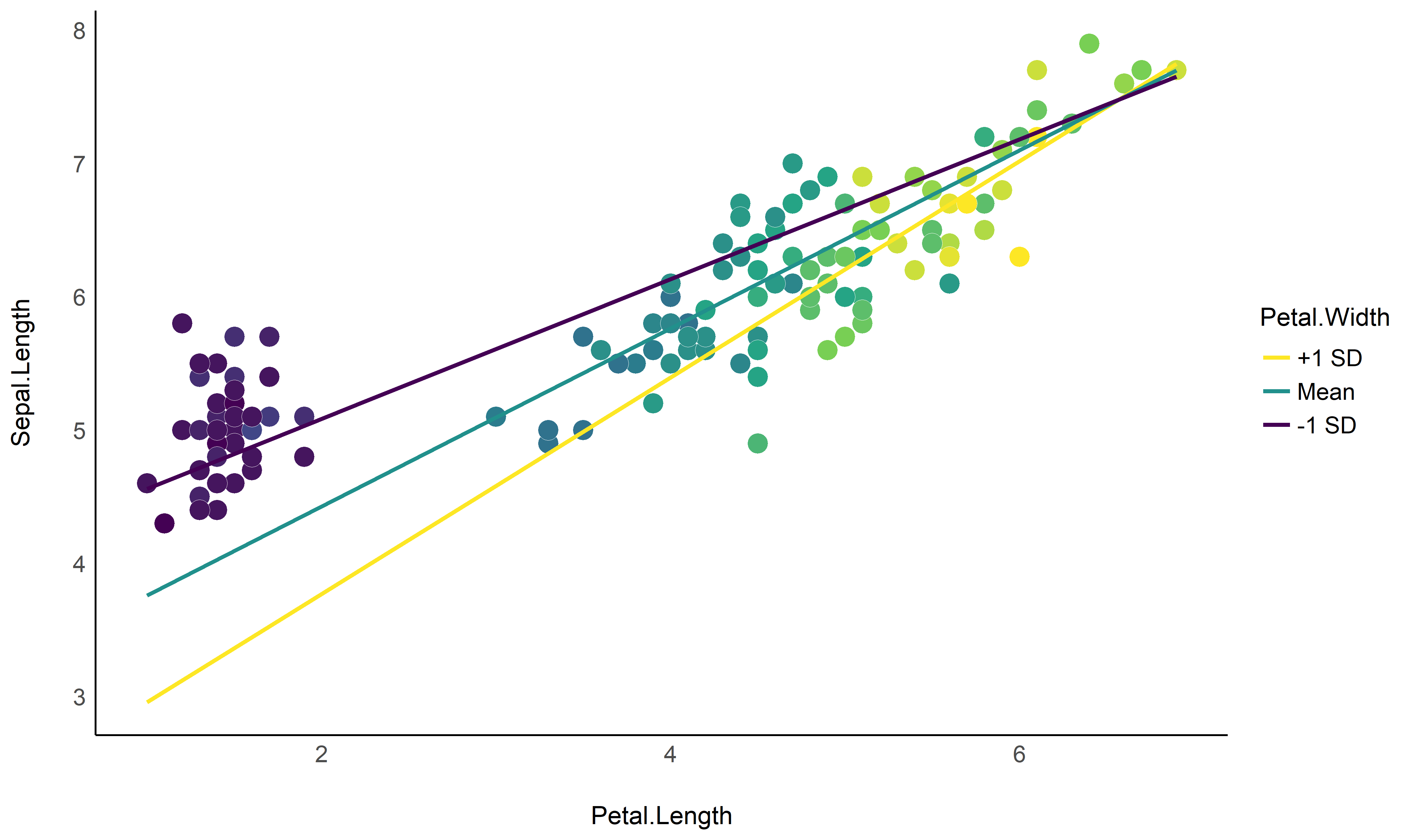
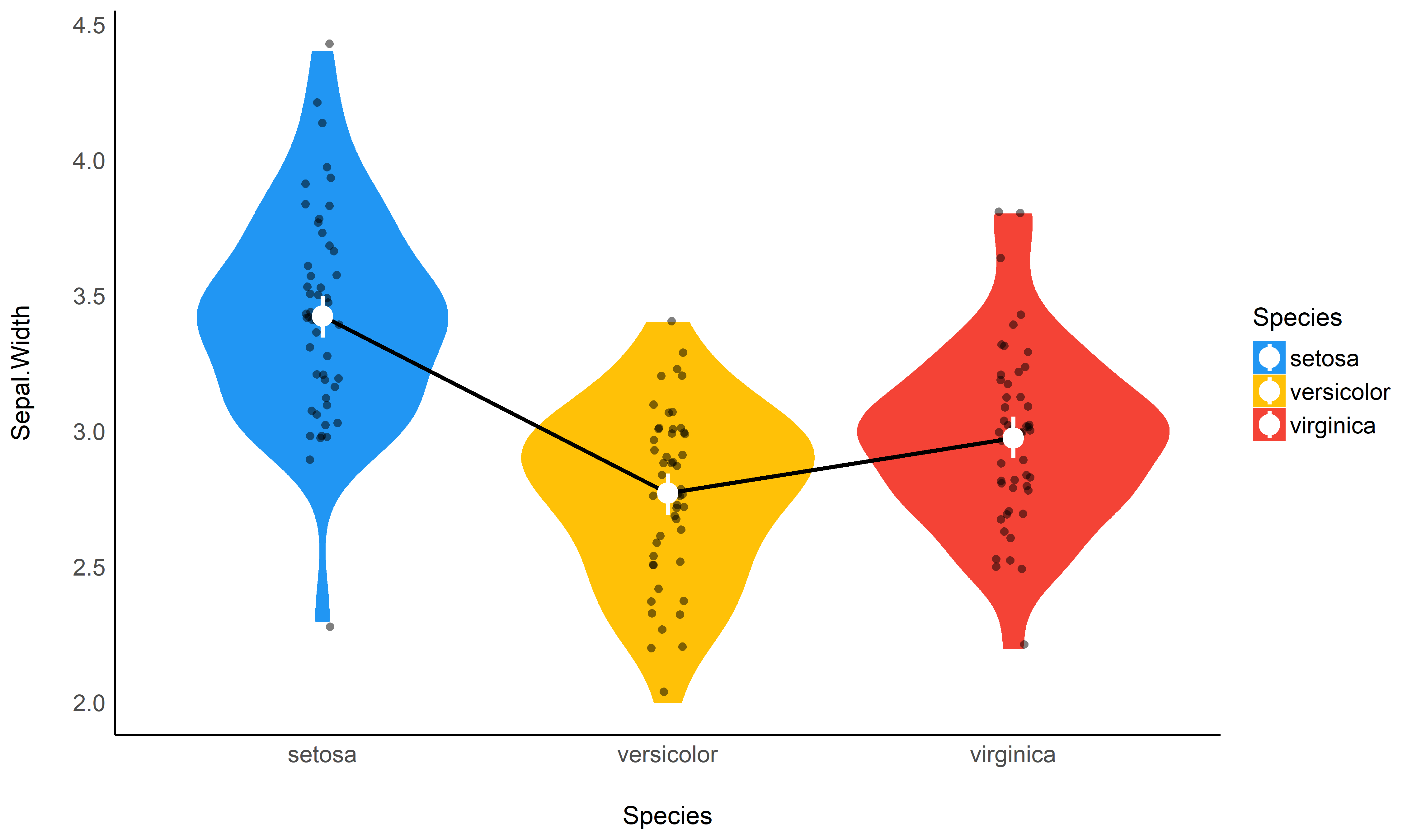
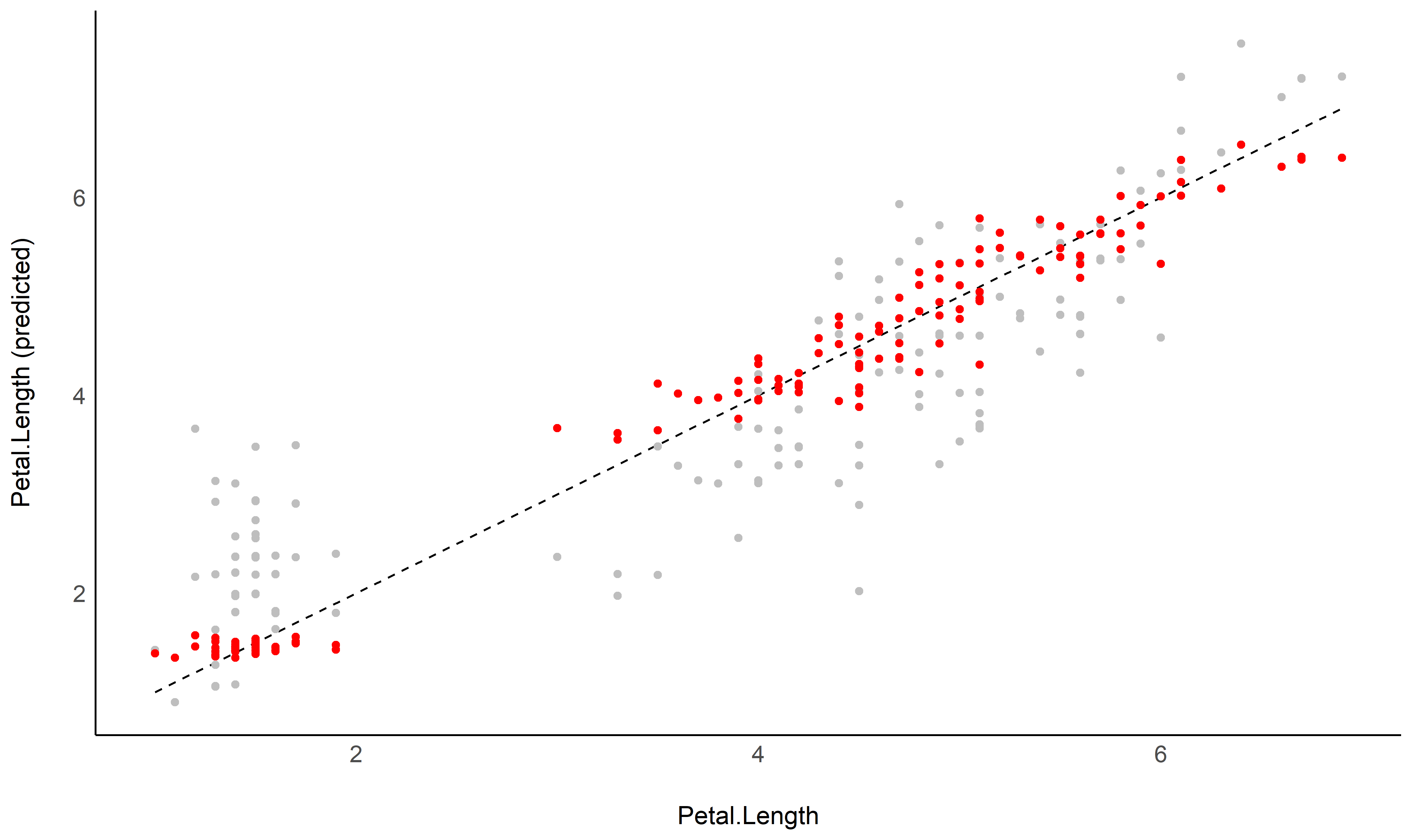
• estimate_means(): Estimates the average values at each factor levels
• estimate_contrasts(): Estimates and tests contrasts between different factor levels
• estimate_slopes(): Estimates the slopes of numeric predictors at different factor levels
• estimate_response(): Predict the response variable using the model
• estimate_smooth(): Describes a non-linear term (e.g. in GAMs) by its linear parts

These functions are powered by the visualisation_matrix() function, a smart tool for guessing the appropriate reference grid.

The package currently only supports rstanarm models, but will be expanded to cover a large variety of frequentist and Bayesian models.

Examples

Create smart grids to represent complex interactions

Check-out this vignette to create this plot:

Estimate marginal means

Check-out this vignette to create this plot:

library(rstanarm)

model <- stan_glm(Sepal.Width ~ Species, data = iris)

estimate_means(model)

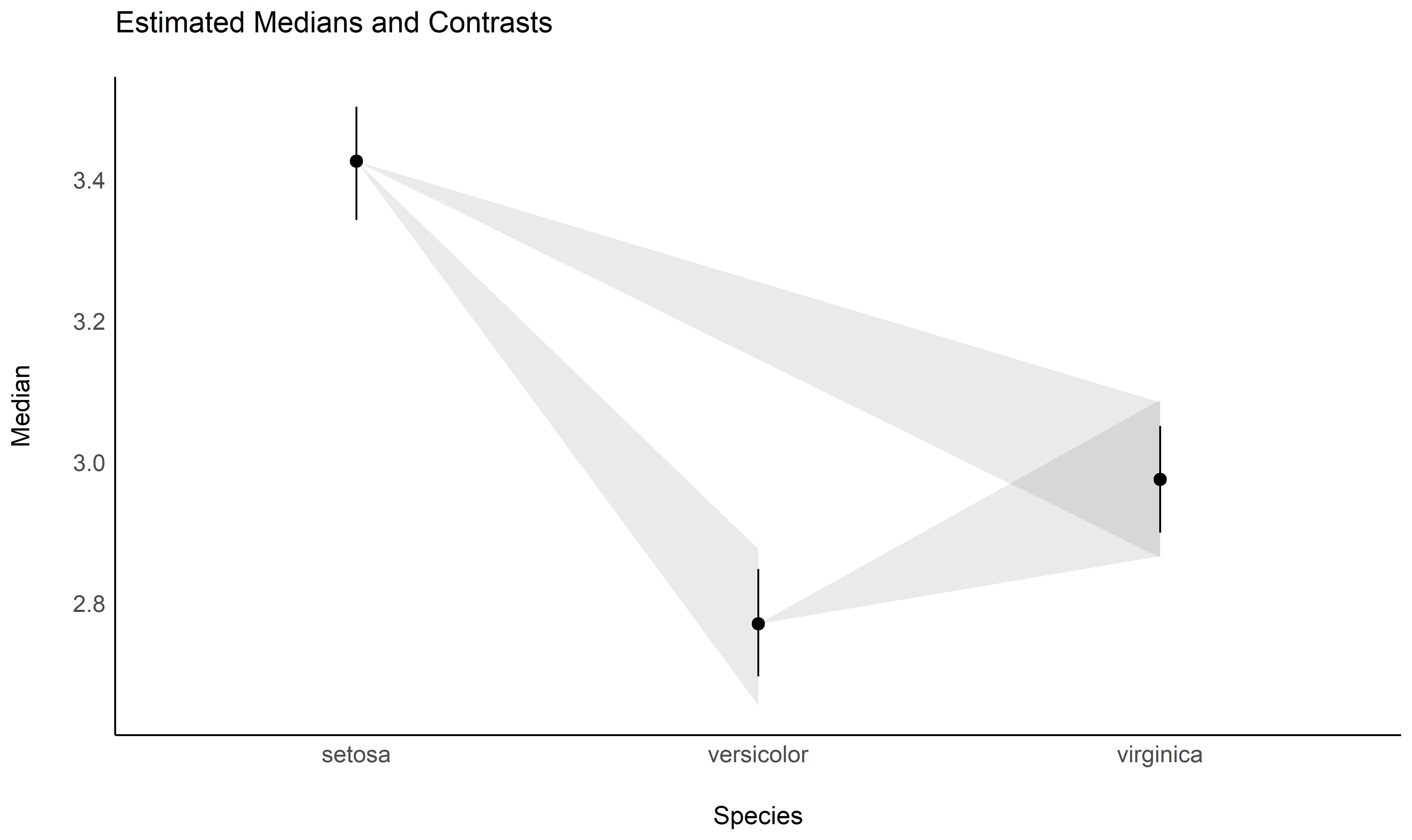
## Species    | Median |       89% CI
## ----------------------------------
## setosa     |   3.43 | [3.34, 3.50]
## versicolor |   2.77 | [2.70, 2.85]
## virginica  |   2.98 | [2.90, 3.05]

Contrast analysis

Check-out this vignette to create this plot:

estimate_contrasts(model)
## Level1     |     Level2 | Median |         89% CI |     pd | % in ROPE | Median (std.)
## --------------------------------------------------------------------------------------
## setosa     | versicolor |   0.65 | [ 0.55,  0.77] |   100% |        0% |          1.50
## setosa     |  virginica |   0.45 | [ 0.34,  0.56] |   100% |        0% |          1.03
## versicolor |  virginica |  -0.21 | [-0.32, -0.10] | 99.83% |     6.93% |         -0.47

Check the contrasts at different points of another linear predictor

model <- stan_glm(Sepal.Width ~ Species * Petal.Length, data = iris)

estimate_contrasts(model, modulate = "Petal.Length", length = 3)

## Level1     |     Level2 | Petal.Length | Median |        89% CI |     pd | % in ROPE | Median (std.)
## ----------------------------------------------------------------------------------------------------
## setosa     | versicolor |         1.00 |   1.52 | [ 1.05, 2.00] |   100% |        0% |          3.48
## setosa     |  virginica |         1.00 |   1.23 | [ 0.69, 1.76] |   100% |     0.02% |          2.82
## versicolor |  virginica |         1.00 |  -0.30 | [-1.03, 0.39] | 74.30% |    13.90% |         -0.68
## setosa     | versicolor |         3.95 |   1.79 | [ 1.04, 2.53] |   100% |        0% |          4.11
## setosa     |  virginica |         3.95 |   1.83 | [ 1.03, 2.60] |   100% |        0% |          4.21
## versicolor |  virginica |         3.95 |   0.04 | [-0.18, 0.26] | 61.40% |    51.00% |          0.09
## setosa     | versicolor |         6.90 |   2.08 | [ 0.50, 3.73] | 98.10% |     1.18% |          4.77
## setosa     |  virginica |         6.90 |   2.45 | [ 0.80, 3.95] | 99.25% |     0.42% |          5.61
## versicolor |  virginica |         6.90 |   0.37 | [-0.06, 0.78] | 91.25% |    11.97% |          0.85

Find a predictor’s slopes at each factor level

estimate_slopes(model)
## Species    | Median |       89% CI |     pd | % in ROPE | Median (std.)
## -----------------------------------------------------------------------
## setosa     |   0.42 | [0.10, 0.69] | 98.85% |     4.10% |          1.70
## versicolor |   0.33 | [0.19, 0.47] | 99.95% |     0.57% |          1.32
## virginica  |   0.21 | [0.09, 0.33] | 99.83% |     6.95% |          0.87

Generate predictions from your model to compare it with original data

Check-out this vignette to create this plot:

estimate_response(model)

Estimate the link between the response and a predictor

See this vignette to create this plot:

model <- stan_glm(Sepal.Width ~ poly(Petal.Length, 2), data=iris)

estimate_link(model)

Describe the smooth term by its linear parts

estimate_smooth(model)
## Part | Start |  End |   Size | Trend | Linearity
## ------------------------------------------------
## 1    |  1.00 | 4.14 | 53.50% | -0.01 |      0.94
## 2    |  4.14 | 6.90 | 46.50% |  0.01 |      0.94