ledger is an R package to import data from plain text accounting software like Ledger, HLedger, and Beancount into an R data frame for convenient analysis, plotting, and export.
Right now it supports reading in the register from ledger, hledger, and beancount files.
To install the last version released to CRAN use the following command in R:
To install the development version of the ledger package (and its R package dependencies) use the install_github function from the remotes package in R:
This package also has some system dependencies that need to be installed depending on which plaintext accounting files you wish to read to be able to read in:
To install hledger run the following in your shell:
stack update && stack install --resolver=lts-14.3 hledger-lib-1.15.2 hledger-1.15.2 hledger-web-1.15 hledger-ui-1.15 --verbosity=error To install beancount run the following in your shell:
Several pre-compiled Ledger binaries are available (often found in several open source repos).
To run the unit tests you'll also need the suggested R package testthat.
The main function of this package is register which reads in the register of a plaintext accounting file. This package also exports S3 methods so one can use rio::import to read in a register, a net_worth convenience function, and a prune_coa convenience function.
Here are some examples of very basic files stored within the package:
library("ledger")
options(width=180)
ledger_file <- system.file("extdata", "example.ledger", package = "ledger")
register(ledger_file)
## # A tibble: 42 x 8
## date mark payee description account amount commodity comment
## <date> <chr> <chr> <chr> <chr> <dbl> <chr> <chr>
## 1 2015-12-31 * <NA> Opening Balances Assets:JT-Checking 5000 USD <NA>
## 2 2015-12-31 * <NA> Opening Balances Equity:Opening -5000 USD <NA>
## 3 2016-01-01 * Landlord Rent Assets:JT-Checking -1500 USD <NA>
## 4 2016-01-01 * Landlord Rent Expenses:Shelter:Rent 1500 USD <NA>
## 5 2016-01-01 * Brokerage Buy Stock Assets:JT-Checking -1000 USD <NA>
## 6 2016-01-01 * Brokerage Buy Stock Equity:Transfer 1000 USD <NA>
## 7 2016-01-01 * Brokerage Buy Stock Assets:JT-Brokerage 4 SP <NA>
## 8 2016-01-01 * Brokerage Buy Stock Equity:Transfer -1000 USD <NA>
## 9 2016-01-01 * Supermarket Grocery store ;; Link: ^grocery Expenses:Food:Grocery 501. USD <NA>
## 10 2016-01-01 * Supermarket Grocery store ;; Link: ^grocery Liabilities:JT-Credit-Card -501. USD <NA>
## # … with 32 more rowshledger_file <- system.file("extdata", "example.hledger", package = "ledger")
register(hledger_file)## # A tibble: 42 x 11
## date mark payee description account amount commodity historical_cost hc_commodity market_value mv_commodity
## <date> <chr> <chr> <chr> <chr> <dbl> <chr> <dbl> <chr> <dbl> <chr>
## 1 2015-12-31 * <NA> Opening Balances Assets:JT-Checking 5000 USD 5000 USD 5000 USD
## 2 2015-12-31 * <NA> Opening Balances Equity:Opening -5000 USD -5000 USD -5000 USD
## 3 2016-01-01 * Landlord Rent Assets:JT-Checking -1500 USD -1500 USD -1500 USD
## 4 2016-01-01 * Landlord Rent Expenses:Shelter:Rent 1500 USD 1500 USD 1500 USD
## 5 2016-01-01 * Brokerage Buy Stock Assets:JT-Checking -1000 USD -1000 USD -1000 USD
## 6 2016-01-01 * Brokerage Buy Stock Equity:Transfer 1000 USD 1000 USD 1000 USD
## 7 2016-01-01 * Brokerage Buy Stock Assets:JT-Brokerage 4 SP 1000 USD 2000 USD
## 8 2016-01-01 * Brokerage Buy Stock Equity:Transfer -1000 USD -1000 USD -1000 USD
## 9 2016-01-01 * Supermarket Grocery store Expenses:Food:Grocery 501. USD 501. USD 501. USD
## 10 2016-01-01 * Supermarket Grocery store Liabilities:JT-Credit-Card -501. USD -501. USD -501. USD
## # … with 32 more rowsbeancount_file <- system.file("extdata", "example.beancount", package = "ledger")
register(beancount_file)## # A tibble: 42 x 12
## date mark payee description account amount commodity historical_cost hc_commodity market_value mv_commodity tags
## <chr> <chr> <chr> <chr> <chr> <dbl> <chr> <dbl> <chr> <dbl> <chr> <chr>
## 1 2015-12-31 * "" Opening Balances Assets:JT-Checking 5000 USD 5000 USD 5000 USD ""
## 2 2015-12-31 * "" Opening Balances Equity:Opening -5000 USD -5000 USD -5000 USD ""
## 3 2016-01-01 * Landlord Rent Assets:JT-Checking -1500 USD -1500 USD -1500 USD ""
## 4 2016-01-01 * Landlord Rent Expenses:Shelter:Rent 1500 USD 1500 USD 1500 USD ""
## 5 2016-01-01 * Brokerage Buy Stock Assets:JT-Checking -1000 USD -1000 USD -1000 USD ""
## 6 2016-01-01 * Brokerage Buy Stock Equity:Transfer 1000 USD 1000 USD 1000 USD ""
## 7 2016-01-01 * Brokerage Buy Stock Assets:JT-Brokerage 4 SP 1000 USD 2000 USD ""
## 8 2016-01-01 * Brokerage Buy Stock Equity:Transfer -1000 USD -1000 USD -1000 USD ""
## 9 2016-01-01 * Supermarket Grocery store Expenses:Food:Grocery 501. USD 501. USD 501. USD ""
## 10 2016-01-01 * Supermarket Grocery store Liabilities:JT-Credit-Card -501. USD -501. USD -501. USD ""
## # … with 32 more rowsHere is an example reading in a beancount file generated by bean-example:
bean_example_file <- tempfile(fileext = ".beancount")
system(paste("bean-example -o", bean_example_file), ignore.stderr=TRUE)
df <- register(bean_example_file)
options(width=240)
print(df)
## # A tibble: 3,206 x 12
## date mark payee description account amount commodity historical_cost hc_commodity market_value mv_commodity tags
## <chr> <chr> <chr> <chr> <chr> <dbl> <chr> <dbl> <chr> <dbl> <chr> <chr>
## 1 2017-01-01 * "" Opening Balance for checking account Assets:US:BofA:Checking 3682. USD 3682. USD 3682. USD ""
## 2 2017-01-01 * "" Opening Balance for checking account Equity:Opening-Balances -3682. USD -3682. USD -3682. USD ""
## 3 2017-01-01 * "" Allowed contributions for one year Income:US:Federal:PreTax401k -18500 IRAUSD -18500 IRAUSD -18500 IRAUSD ""
## 4 2017-01-01 * "" Allowed contributions for one year Assets:US:Federal:PreTax401k 18500 IRAUSD 18500 IRAUSD 18500 IRAUSD ""
## 5 2017-01-03 * RiverBank Properties Paying the rent Assets:US:BofA:Checking -2400 USD -2400 USD -2400 USD ""
## 6 2017-01-03 * RiverBank Properties Paying the rent Expenses:Home:Rent 2400 USD 2400 USD 2400 USD ""
## 7 2017-01-04 * BANK FEES Monthly bank fee Assets:US:BofA:Checking -4 USD -4 USD -4 USD ""
## 8 2017-01-04 * BANK FEES Monthly bank fee Expenses:Financial:Fees 4 USD 4 USD 4 USD ""
## 9 2017-01-05 * Uncle Boons Eating out with Julie Liabilities:US:Chase:Slate -58.9 USD -58.9 USD -58.9 USD ""
## 10 2017-01-05 * Uncle Boons Eating out with Julie Expenses:Food:Restaurant 58.9 USD 58.9 USD 58.9 USD ""
## # … with 3,196 more rowssuppressPackageStartupMessages(library("dplyr"))
dplyr::filter(df, grepl("Expenses", account), grepl("trip", tags)) %>%
group_by(trip = tags, account) %>%
summarise(trip_total = sum(amount))## # A tibble: 7 x 3
## # Groups: trip [3]
## trip account trip_total
## <chr> <chr> <dbl>
## 1 trip-boston-2019 Expenses:Food:Coffee 29.2
## 2 trip-boston-2019 Expenses:Food:Restaurant 425.
## 3 trip-chicago-2018 Expenses:Food:Alcohol 47.5
## 4 trip-chicago-2018 Expenses:Food:Coffee 28.0
## 5 trip-chicago-2018 Expenses:Food:Restaurant 602
## 6 trip-san-francisco-2017 Expenses:Food:Coffee 35.1
## 7 trip-san-francisco-2017 Expenses:Food:Restaurant 700.If one has loaded in the ledger package one can also use rio::import to read in the register:
## Unrecognized file format. Try specifying with the format argument.## Unrecognized file format. Try specifying with the format argument.
## [1] TRUEThe main advantage of this is that it allows one to use rio::convert to easily convert plaintext accounting files to several other file formats such as a csv file. Here is a shell example:
bean-example -o example.beancount
Rscript --default-packages=ledger,rio -e 'convert("example.beancount", "example.csv")'Some examples of using the net_worth function using the example files from the register examples:
dates <- seq(as.Date("2016-01-01"), as.Date("2018-01-01"), by="years")
net_worth(ledger_file, dates)
## # A tibble: 3 x 6
## date commodity net_worth assets liabilities revalued
## <date> <chr> <dbl> <dbl> <dbl> <dbl>
## 1 2016-01-01 USD 5000 5000 0 0
## 2 2017-01-01 USD 4361. 4882 -521. 0
## 3 2018-01-01 USD 6743. 6264 -521. 1000## # A tibble: 3 x 5
## date commodity net_worth assets liabilities
## <date> <chr> <dbl> <dbl> <dbl>
## 1 2016-01-01 USD 5000 5000 0
## 2 2017-01-01 USD 4361. 4882 -521.
## 3 2018-01-01 USD 6743. 7264 -521.## # A tibble: 3 x 5
## date commodity net_worth assets liabilities
## <date> <chr> <dbl> <dbl> <dbl>
## 1 2016-01-01 USD 5000 5000 0
## 2 2017-01-01 USD 4361. 4882 -521.
## 3 2018-01-01 USD 6743. 7264 -521.## # A tibble: 3 x 5
## date commodity net_worth assets liabilities
## <date> <chr> <dbl> <dbl> <dbl>
## 1 2018-01-01 IRAUSD 0 0 0
## 2 2018-01-01 USD 40382. 41529. -1147.
## 3 2018-01-01 VACHR 34 34 0Some examples using the prune_coa function to simplify the "Chart of Account" names to a given maximum depth:
suppressPackageStartupMessages(library("dplyr"))
df <- register(bean_example_file) %>% dplyr::filter(!is.na(commodity))
df %>% prune_coa() %>%
    group_by(account, mv_commodity) %>%
    summarize(market_value = sum(market_value))
## # A tibble: 11 x 3
## # Groups: account [5]
## account mv_commodity market_value
## <chr> <chr> <dbl>
## 1 Assets IRAUSD 0
## 2 Assets USD 109301.
## 3 Assets VACHR -2
## 4 Equity USD -3682.
## 5 Expenses IRAUSD 55500
## 6 Expenses USD 252946.
## 7 Expenses VACHR 352
## 8 Income IRAUSD -55500
## 9 Income USD -353352.
## 10 Income VACHR -350
## 11 Liabilities USD -2926.df %>% prune_coa(2) %>%
group_by(account, mv_commodity) %>%
summarize(market_value = sum(market_value))## # A tibble: 17 x 3
## # Groups: account [12]
## account mv_commodity market_value
## <chr> <chr> <dbl>
## 1 Assets:US IRAUSD 0.
## 2 Assets:US USD 1.09e+ 5
## 3 Assets:US VACHR -2.00e+ 0
## 4 Equity:Opening-Balances USD -3.68e+ 3
## 5 Expenses:Financial USD 4.14e+ 2
## 6 Expenses:Food USD 1.78e+ 4
## 7 Expenses:Health USD 6.78e+ 3
## 8 Expenses:Home USD 8.34e+ 4
## 9 Expenses:Taxes IRAUSD 5.55e+ 4
## 10 Expenses:Taxes USD 1.41e+ 5
## 11 Expenses:Transport USD 3.72e+ 3
## 12 Expenses:Vacation VACHR 3.52e+ 2
## 13 Income:US IRAUSD -5.55e+ 4
## 14 Income:US USD -3.53e+ 5
## 15 Income:US VACHR -3.50e+ 2
## 16 Liabilities:AccountsPayable USD 5.68e-14
## 17 Liabilities:US USD -2.93e+ 3Here is some examples using the functions in the package to help generate various personal accounting reports of the beancount example generated by bean-example.
First we load the (mainly tidyverse) libraries we'll be using and adjusting terminal output:
options(width=240) # tibble output looks better in wide terminal output
library("ledger")
library("dplyr")
filter <- dplyr::filter
library("ggplot2")
library("scales")
library("tidyr")
library("zoo")
filename <- tempfile(fileext = ".beancount")
system(paste("bean-example -o", filename), ignore.stderr=TRUE)
df <- register(filename) %>% mutate(yearmon = zoo::as.yearmon(date)) %>%
      filter(commodity=="USD")
nw <- net_worth(filename)
Then we'll write some convenience functions we'll use over and over again:
print_tibble_rows <- function(df) {
    print(df, n=nrow(df))
}
count_beans <- function(df, filter_str = "", ...,
                        amount = "amount",
                        commodity="commodity",
                        cutoff=1e-3) {
    commodity <- sym(commodity)
    amount_var <- sym(amount)
    filter(df, grepl(filter_str, account)) %>%
        group_by(account, !!commodity, ...) %>%
        summarize(!!amount := sum(!!amount_var)) %>%
        filter(abs(!!amount_var) > cutoff & !is.na(!!amount_var)) %>%
        arrange(desc(abs(!!amount_var)))
}Here is some basic balance sheets (using the market value of our assets):
print_balance_sheet <- function(df) {
    assets <- count_beans(df, "^Assets",
                 amount="market_value", commodity="mv_commodity")
    print_tibble_rows(assets)
    liabilities <- count_beans(df, "^Liabilities",
                       amount="market_value", commodity="mv_commodity")
    print_tibble_rows(liabilities)
}
print(nw)
## # A tibble: 3 x 5
## date commodity net_worth assets liabilities
## <date> <chr> <dbl> <dbl> <dbl>
## 1 2019-09-03 IRAUSD 0 0 0
## 2 2019-09-03 USD 118656. 121202. -2546.
## 3 2019-09-03 VACHR 78 78 0## # A tibble: 1 x 3
## # Groups: account [1]
## account mv_commodity market_value
## <chr> <chr> <dbl>
## 1 Assets:US USD 3626.
## # A tibble: 1 x 3
## # Groups: account [1]
## account mv_commodity market_value
## <chr> <chr> <dbl>
## 1 Liabilities:US USD -2546.## # A tibble: 3 x 3
## # Groups: account [3]
## account mv_commodity market_value
## <chr> <chr> <dbl>
## 1 Assets:US:BofA:Checking USD 2946.
## 2 Assets:US:ETrade:Cash USD 680.
## 3 Assets:US:Vanguard:Cash USD 0.11
## # A tibble: 1 x 3
## # Groups: account [1]
## account mv_commodity market_value
## <chr> <chr> <dbl>
## 1 Liabilities:US:Chase:Slate USD -2546.Here is a basic chart of one's net worth from the beginning of the plaintext accounting file to today by month:
next_month <- function(date) {
    zoo::as.Date(zoo::as.yearmon(date) + 1/12)
}
nw_dates <- seq(next_month(min(df$date)), next_month(Sys.Date()), by="months")
df_nw <- net_worth(filename, nw_dates) %>% filter(commodity=="USD")
ggplot(df_nw, aes(x=date, y=net_worth, colour=commodity, group=commodity)) +
  geom_line() + scale_y_continuous(labels=scales::dollar)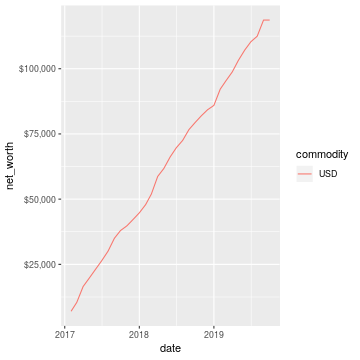
month_cutoff <- zoo::as.yearmon(Sys.Date()) - 2/12
compute_income <- function(df) {
    count_beans(df, "^Income", yearmon) %>%
        mutate(income = -amount) %>%
        select(-amount) %>% ungroup()
}
print_income <- function(df) {
    compute_income(df) %>%
        filter(yearmon >= month_cutoff) %>%
        spread(yearmon, income, fill=0) %>%
        print_tibble_rows()
}
compute_expenses <- function(df) {
    count_beans(df, "^Expenses", yearmon) %>%
        mutate(expenses = amount) %>%
        select(-amount) %>% ungroup()
}
print_expenses <- function(df) {
    compute_expenses(df) %>%
        filter(yearmon >= month_cutoff) %>%
        spread(yearmon, expenses, fill=0) %>%
        print_tibble_rows()
}
compute_total <- function(df) {
full_join(compute_income(prune_coa(df)) %>% select(-account),
          compute_expenses(prune_coa(df)) %>% select(-account),
          by=c("yearmon", "commodity")) %>%
    mutate(income = ifelse(is.na(income), 0, income),
           expenses = ifelse(is.na(expenses), 0, expenses),
           net = income - expenses) %>%
    gather(type, amount, -yearmon, -commodity)
}
print_total <- function(df) {
    compute_total(df) %>%
        filter(yearmon >= month_cutoff) %>%
        spread(yearmon, amount, fill=0) %>%
        print_tibble_rows()
}
print_total(df)
## # A tibble: 3 x 4
## commodity type `Jul 2019` `Aug 2019`
## <chr> <chr> <dbl> <dbl>
## 1 USD expenses 7421. 9528.
## 2 USD income 10479. 14169.
## 3 USD net 3059. 4641.## # A tibble: 1 x 4
## account commodity `Jul 2019` `Aug 2019`
## <chr> <chr> <dbl> <dbl>
## 1 Income:US USD 10479. 14169.## # A tibble: 6 x 4
## account commodity `Jul 2019` `Aug 2019`
## <chr> <chr> <dbl> <dbl>
## 1 Expenses:Financial USD 4 21.9
## 2 Expenses:Food USD 519. 512.
## 3 Expenses:Health USD 194. 291.
## 4 Expenses:Home USD 2600. 2606.
## 5 Expenses:Taxes USD 3984. 5977.
## 6 Expenses:Transport USD 120 120## # A tibble: 3 x 4
## account commodity `Jul 2019` `Aug 2019`
## <chr> <chr> <dbl> <dbl>
## 1 Income:US:Hooli:GroupTermLife USD 48.6 73.0
## 2 Income:US:Hooli:Match401k USD 1200 250
## 3 Income:US:Hooli:Salary USD 9231. 13846.## # A tibble: 19 x 4
## account commodity `Jul 2019` `Aug 2019`
## <chr> <chr> <dbl> <dbl>
## 1 Expenses:Financial:Commissions USD 0 17.9
## 2 Expenses:Financial:Fees USD 4 4
## 3 Expenses:Food:Groceries USD 219. 156.
## 4 Expenses:Food:Restaurant USD 301. 357.
## 5 Expenses:Health:Dental:Insurance USD 5.8 8.7
## 6 Expenses:Health:Life:GroupTermLife USD 48.6 73.0
## 7 Expenses:Health:Medical:Insurance USD 54.8 82.1
## 8 Expenses:Health:Vision:Insurance USD 84.6 127.
## 9 Expenses:Home:Electricity USD 65 65
## 10 Expenses:Home:Internet USD 80.0 79.9
## 11 Expenses:Home:Phone USD 54.5 61.3
## 12 Expenses:Home:Rent USD 2400 2400
## 13 Expenses:Taxes:Y2019:US:CityNYC USD 350. 525.
## 14 Expenses:Taxes:Y2019:US:Federal USD 2126. 3189.
## 15 Expenses:Taxes:Y2019:US:Medicare USD 213. 320.
## 16 Expenses:Taxes:Y2019:US:SDI USD 2.24 3.36
## 17 Expenses:Taxes:Y2019:US:SocSec USD 563. 845.
## 18 Expenses:Taxes:Y2019:US:State USD 730. 1095.
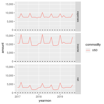
## 19 Expenses:Transport:Tram USD 120 120And here is a plot of income, expenses, and net income over time:
ggplot(compute_total(df), aes(x=yearmon, y=amount, group=commodity, colour=commodity)) +
  facet_grid(type ~ .) +
  geom_line() + geom_hline(yintercept=0, linetype="dashed") +
  scale_x_continuous() + scale_y_continuous(labels=scales::comma)