
![]()

![]()
An R package for univariate kernel density estimation with parametric starts and asymmetric kernels.
kdensity is an implementation of univariate kernel density estimation with support for parametric starts and asymmetric kernels. Its main function is kdensity, which is has approximately the same syntax as stats::density. Its new functionality is:
kdensity has built-in support for many parametric starts, such as normal and gamma, but you can also supply your own.gcopula and gamma kernels, but also the common symmetric ones. In addition, you can also supply your own kernels.bw, again including an option to specify your own.A reason to use kdensity is to avoid boundary bias when estimating densities on the unit interval or the positive half-line. Asymmetric kernels such as gamma and gcopula are designed for this purpose. The support for parametric starts allows you to easily use a method that is often superior to ordinary kernel density estimation.
From inside R, use one of the following commands:
# For the CRAN release
install.packages("kdensity")
# For the development version from GitHub:
# install.packages("devtools")
devtools::install_github("JonasMoss/kdensity")
Call the library function and use it just like stats:density, but with optional additional arguments.
Kernel density estimation with a parametric start was introduced by Hjort and Glad in Nonparametric Density Estimation with a Parametric Start (1995). The idea is to start out with a parametric density before you do your kernel density estimation, so that your actual kernel density estimation will be a correction to the original parametric estimate. This is a good idea because the resulting estimator will be better than an ordinary kernel density estimator whenever the true density is close to your suggestion; and the estimator can be superior to the ordinary kernel density estimator even when the suggestion is pretty far off.
In addition to parametric starts, the package implements some asymmetric kernels. These kernels are useful when modelling data with sharp boundaries, such as data supported on the positive half-line or the unit interval. Currently we support the following asymmetric kernels:
Jones and Henderson’s Gaussian copula KDE, from Kernel-Type Density Estimation on the Unit Interval (2007). This is used for data on the unit interval. The bandwidth selection mechanism described in that paper is implemented as well. This kernel is called gcopula.
Chen’s two beta kernels from Beta kernel estimators for density functions (1999). These are used for data supported on the on the unit interval, and are called beta and beta_biased.
Chen’s two gamma kernels from Probability Density Function Estimation Using Gamma Kernels (2000). These are used for data supported on the positive half-line, and are called gamma and gamma_biased.
These features can be combined to make asymmetric kernel densities estimators with parametric starts, see the example below. The package contains only one function, kdensity, in addition to the generics plot, points, lines, summary, and print.
The function kdensity takes some data, a kernel kernel and a parametric start start. You can optionally specify the support parameter, which is used to find the normalizing constant.
The following example uses the data set plots both a gamma-kernel density estimate with a gamma start (black) and the the fully parametric gamma density. The underlying parameter estimates are always maximum likelood.
library("kdensity")
kde = kdensity(airquality$Wind, start = "gamma", kernel = "gamma")
plot(kde, main = "Wind speed (mph)")
lines(kde, plot_start = TRUE, col = "red")
rug(airquality$Wind)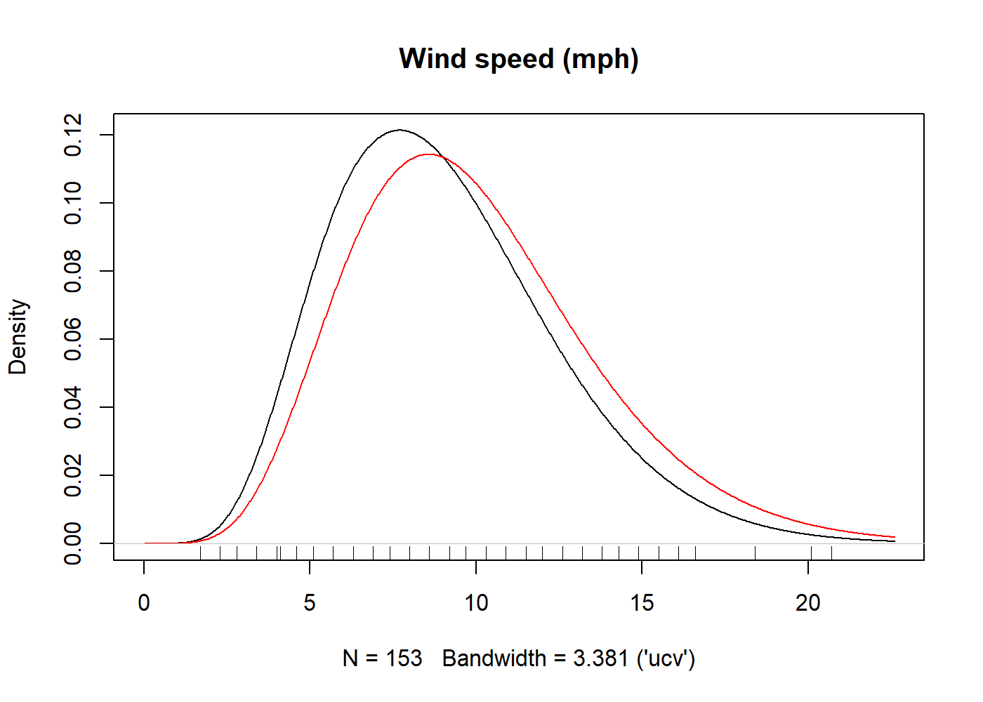
Since the return value of kdensity is a function, it is callable, as in:
You can access the parameter estimates by using coef. You can also access the log likelihood (logLik), AIC and BIC of the parametric start distribution.
coef(kde)
#>     shape      rate
#> 7.1872898 0.7217954
logLik(kde)
#> 'log Lik.' 12.33787 (df=2)
AIC(kde)
#> [1] -20.67574