The goal of irtplay is to fit unidimensional item response theory (IRT) models to mixture of dichotomous and polytomous data, calibrate online item parameters (i.e., pretest and operational items), estimate examinees abilities, and examine the IRT model-data fit on item-level in different ways as well as provide useful functions related to unidimensional IRT.
For the item parameter estimation, the marginal maximum likelihood estimation with expectation-maximization (MMLE-EM) algorithm (Bock & Aitkin, 1981) is used. For the online calibration, Stocking’s Method A (Ban, Hanson, Wang, Yi, & Harris, 2001; stocking, 1988) and the fixed item parameter calibration (FIPC) method (Kim, 2006) are provided. For the ability estimation, several popular scoring methods (e.g., MLE, EAP, and MAP) are implemented. In terms of assessing the IRT model-data fit, one of distinguished features of this package is that it gives not only item fit statistics (e.g., chi-square fit statistic (X2; e.g., Bock, 1960; Yen, 1981), likelihood ratio chi-square fit statistic (G2; McKinley & Mills, 1985), infit and outfit statistics (Ames et al., 2015), and S-X2 (Orlando & Thissen, 2000, 2003)) but also graphical displays to look at residuals between the observed data and model-based predictions (Hambleton, Swaminathan, & Rogers, 1991).
In addition, there are many useful functions such as computing asymptotic variance-covariance matrices of item parameter estimates, importing item and/or ability parameters from popular IRT software, running flexMIRT (Cai, 2017) through R, generating simulated data, computing the conditional distribution of observed scores using the Lord-Wingersky recursion formula, computing item and test information functions, computing item and test characteristic curve functions, and plotting item and test characteristic curves and item and test information functions.
You can install the released version of irtplay from CRAN with:
The fixed item parameter calibration (FIPC) is one of useful online item calibration methods for computerized adaptive testing (CAT) to put the parameter estimates of pretest items on the same scale of operational item parameter estimates without post hoc linking/scaling (Ban, Hanson, Wang, Yi, & Harris, 2001; Chen & Wang, 2016). In FIPC, the operational item parameters are fixed to estimate the characteristic of the underlying latent variable prior distribution when calibrating the pretest items. More specifically, the underlying latent variable prior distribution of the operational items is estimated during the calibration of the pretest items to put the item parameters of the pretest items on the scale of the operational item parameters (Kim, 2006). In irtplay package, FIPC is implemented with two main steps:
est_irt function.To run the est_irt function, it requires two data sets:
x in the function est_irt).When FIPC is implemented in est_irt function, the pretest item parameters are estimated by fixing the operational item parameters. To estimate the item parameters, you need to provide the item meta data in the argument x and the response data in the argument data.
It is worthwhile to explain about how to prepare the item meta data set in the argument x. A specific form of a data.frame should be used for the argument x. The first column should have item IDs, the second column should contain the number of score categories of the items, and the third column should include IRT models. The available IRT models are “1PLM”, “2PLM”, “3PLM”, and “DRM” for dichotomous items, and “GRM” and “GPCM” for polytomous items. Note that “DRM” covers all dichotomous IRT models (i.e, “1PLM”, “2PLM”, and “3PLM”) and “GRM” and “GPCM” represent the graded response model and (generalized) partial credit model, respectively. From the fourth column, item parameters should be included. For dichotomous items, the fourth, fifth, and sixth columns represent the item discrimination (or slope), item difficulty, and item guessing parameters, respectively. When “1PLM” or “2PLM” is specified for any items in the third column, NAs should be inserted for the item guessing parameters. For polytomous items, the item discrimination (or slope) parameters should be contained in the fourth column and the item threshold (or step) parameters should be included from the fifth to the last columns. When the number of categories differs between items, the empty cells of item parameters should be filled with NAs. See est_irt for more details about the item meta data.
Also, you should specify in the argument ’fipc = TRUEand a specific FIPC method in the argumentfipc.method. Finally, you should provide a vector of the location of the items to be fixed in the argumentfix.loc. For more details about implementing FIPC, see the description of the functionest_irt`.
When implementing FIPC, you can estimate both the emprical histogram and the scale of latent variable prior distribution by setting EmpHist = TRUE. If EmpHist = FALSE, the normal prior distribution is used during the item parameter estimation and the scale of the normal prior distribution is updated during the EM cycle.
If necessary, you need to specify whether prior distributions of item slope and guessing parameters (only for the IRT 3PL model) are used in the arguments of use.aprior and use.gprior, respectively. If you decide to use the prior distributions, you should specify what distributions will be used for the prior distributions in the arguments of aprior and gprior, respectively. Currently three probability distributions of Beta, Log-normal, and Normal distributions are available.
In addition, if the response data include missing values, you must indicate the missing value in argument missing.
Once the est_irt function has been implemented, you’ll get a list of several internal objects such as the item parameter estimates, standard error of the parameter estimates.
In CAT, Method A is the relatively simplest and most straightforward online calibration method, which is the maximum likelihood estimation of the item parameters given the proficiency estimates. In CAT, Method A can be used to put the parameter estimates of pretest items on the same scale of operational item parameter estimates and recalibrate the operational items to evaluate the parameter drifts of the operational items (Chen & Wang, 2016; Stocking, 1988). Also, Method A is known to result in accurate, unbiased item parameters calibration when items are randomly rather than adaptively administered to examinees, which occurs most commonly with pretest items (Ban et al., 2001; Chen & Wang, 2016). Using irtplay package, Method A is implemented to calibrate the items with two main steps:
est_item function.To run the est_item function, it requires two data sets:
The est_item function estimates the pretest item parameters given the proficiency estimates. To estimate the item parameters, you need to provide the response data in the argument data and the ability estimates in the argument score.
Also, you should provide a string vector of the IRT models in the argument model to indicate what IRT model is used to calibrate each item. Available IRT models are “1PLM”, “2PLM”, “3PLM”, and “DRM” for dichotomous items, and “GRM” and “GPCM” for polytomous items. “GRM” and “GPCM” represent the graded response model and (generalized) partial credit model, respectively. Note that “DRM” is considered as “3PLM” in this function. If a single character of the IRT model is specified, that model will be recycled across all items.
The est_item function requires a vector of the number of score categories for the items in the argument cats. For example, a dichotomous item has two score categories. If a single numeric value is specified, that value will be recycled across all items. If NULL and all items are binary items (i.e., dichotomous items), it assumes that all items have two score categories.
If necessary, you need to specify whether prior distributions of item slope and guessing parameters (only for the IRT 3PL model) are used in the arguments of use.aprior and use.gprior, respectively. If you decide to use the prior distributions, you should specify what distributions will be used for the prior distributions in the arguments of aprior and gprior, respectively. Currently three probability distributions of Beta, Log-normal, and Normal distributions are available.
In addition, if the response data include missing values, you must indicate the missing value in argument missing.
Once the est_item function has been implemented, you’ll get a list of several internal objects such as the item parameter estimates, standard error of the parameter estimates.
One way to assess goodness of IRT model-data fit is through an item fit analysis by examining the traditional item fit statistics and looking at the discrepancy between the observed data and model-based predictions. Using irtplay package, the traditional approach of evaluating the IRT model-data fit on item-level can be implemented with three main steps:
irtfit function.irtfit) obtained in step 2, draw the IRT residual plots (i.e., raw residual and standardized residual plots) using plot method.Before conducting the IRT model fit analysis, it is necessary to prepare a data set. To run the irtfit function, it requires three data sets:
shape_df function or by creating a data.frame of the item meta data by yourself. If you have output files of item parameter estimates obtained from one of the IRT software such as BILOG-MG 3, PARSCALE 4, flexMIRT, and mirt (R package), the item meta data can be easily obtained using the functions of bring.bilog, bring.parscale, bring.flexmirt, bring.mirt. See the functions of irtfit, test.info, or simdat for more details about the item meta data format.The irtfit function computes the traditional IRT item fit statistics such as X2, G2, infit, and outfit statistics. To calculate the X2 and G2 statistics, two methods are available to divide the ability scale into several groups. The two methods are “equal.width” for dividing the scale by an equal length of the interval and “equal.freq” for dividing the scale by an equal frequency of examinees. Also, you need to specify the location of ability point at each group (or interval) where the expected probabilities of score categories are calculated from the IRT models. Available locations are “average” for computing the expected probability at the average point of examinees’ ability estimates in each group and “middle” for computing the expected probability at the midpoint of each group.
To use the irtfit function, you need to insert the item meta data in the argument x, the ability estimates in the argument score, and the response data in the argument data. If you want to divide the ability scale into other than ten groups, you need to specify the number of groups in the argument n.width. In addition, if the response data include missing values, you must indicate the missing value in argument missing.
Once the irtfit function has been implemented, you’ll get the fit statistic results and the contingency tables for every item used to calculate the X2 and G2 fit statistics.
Using the saved object of class irtfit, you can use the plot method to evaluate the IRT raw residual and standardized residual plots.
Because the plot method can draw the residual plots for an item at a time, you have to indicate which item will be examined. For this, you can specify an integer value, which is the location of the studied item, in the argument item.loc.
In terms of the raw residual plot, the argument ci.method is used to select a method to estimate the confidence intervals among four methods. Those methods are “wald” for the Wald interval, which is based on the normal approximation (Laplace, 1812), “cp” for Clopper-Pearson interval (Clopper & Pearson, 1934), “wilson” for Wilson score interval (Wilson, 1927), and “wilson.cr” for Wilson score interval with continuity correction (Newcombe, 1998).
library(irtplay)
##----------------------------------------------------------------------------
# 1. The example code below shows how to prepare the data sets and how to
# implement the fixed item parameter calibration (FIPC):
##----------------------------------------------------------------------------
## Step 1: prepare a data set
## In this example, we generated examinees' true proficiency parameters and simulated
## the item response data using the function "simdat".
## import the "-prm.txt" output file from flexMIRT
flex_sam <- system.file("extdata", "flexmirt_sample-prm.txt", package = "irtplay")
# select the item meta data
x <- bring.flexmirt(file=flex_sam, "par")$Group1$full_df
# generate 1,000 examinees' latent abilities from N(0.4, 1.3)
set.seed(20)
score <- rnorm(1000, mean=0.4, sd=1.3)
# simulate the response data
sim.dat <- simdat(x=x, theta=score, D=1)
## Step 2: Estimate the item parameters
# fit the 3PL model to all dichotmous items, fit the GRM model to all polytomous data,
# fix the five 3PL items (1st - 5th items) and three GRM items (53th to 55th items)
# also, estimate the empirical histogram of latent variable
fix.loc <- c(1:5, 53:55)
(mod.fix1 <- est_irt(x=x, data=sim.dat, D=1, use.gprior=TRUE, gprior=list(dist="beta", params=c(5, 16)),
EmpHist=TRUE, Etol=1e-3, fipc=TRUE, fipc.method="MEM", fix.loc=fix.loc))
#> Parsing input...
#> Estimating item parameters...
#> EM iteration: 1, Loglike: -28912.3526, Max-Change: 3.22265 EM iteration: 2, Loglike: -25094.9221, Max-Change: 0.86707 EM iteration: 3, Loglike: -24854.5695, Max-Change: 0.23789 EM iteration: 4, Loglike: -24847.9987, Max-Change: 0.09966 EM iteration: 5, Loglike: -24846.7185, Max-Change: 0.0740 EM iteration: 6, Loglike: -24846.1673, Max-Change: 0.05455 EM iteration: 7, Loglike: -24845.8645, Max-Change: 0.04023 EM iteration: 8, Loglike: -24845.6791, Max-Change: 0.02986 EM iteration: 9, Loglike: -24845.5582, Max-Change: 0.02239 EM iteration: 10, Loglike: -24845.4763, Max-Change: 0.01698 EM iteration: 11, Loglike: -24845.4193, Max-Change: 0.01302 EM iteration: 12, Loglike: -24845.3793, Max-Change: 0.01048 EM iteration: 13, Loglike: -24845.3513, Max-Change: 0.00898 EM iteration: 14, Loglike: -24845.3319, Max-Change: 0.0083 EM iteration: 15, Loglike: -24845.3191, Max-Change: 0.00759 EM iteration: 16, Loglike: -24845.3112, Max-Change: 0.00689 EM iteration: 17, Loglike: -24845.3072, Max-Change: 0.00623 EM iteration: 18, Loglike: -24845.3061, Max-Change: 0.00562 EM iteration: 19, Loglike: -24845.3075, Max-Change: 0.00506 EM iteration: 20, Loglike: -24845.3108, Max-Change: 0.00455 EM iteration: 21, Loglike: -24845.3156, Max-Change: 0.00409 EM iteration: 22, Loglike: -24845.3217, Max-Change: 0.00369 EM iteration: 23, Loglike: -24845.3288, Max-Change: 0.00332 EM iteration: 24, Loglike: -24845.3367, Max-Change: 0.00299 EM iteration: 25, Loglike: -24845.3453, Max-Change: 0.0027 EM iteration: 26, Loglike: -24845.3544, Max-Change: 0.00244 EM iteration: 27, Loglike: -24845.3641, Max-Change: 0.00221 EM iteration: 28, Loglike: -24845.3740, Max-Change: 0.0020 EM iteration: 29, Loglike: -24845.3843, Max-Change: 0.00181 EM iteration: 30, Loglike: -24845.3948, Max-Change: 0.00164 EM iteration: 31, Loglike: -24845.4055, Max-Change: 0.00149 EM iteration: 32, Loglike: -24845.4163, Max-Change: 0.00135 EM iteration: 33, Loglike: -24845.4273, Max-Change: 0.00123 EM iteration: 34, Loglike: -24845.4383, Max-Change: 0.00111 EM iteration: 35, Loglike: -24845.4493, Max-Change: 0.00101 EM iteration: 36, Loglike: -24845.4604, Max-Change: 0.00092
#> Computing item parameter var-covariance matrix...
#> Estimation is finished in 6.79 seconds.
#>
#> Call:
#> est_irt(x = x, data = sim.dat, D = 1, use.gprior = TRUE, gprior = list(dist = "beta",
#> params = c(5, 16)), EmpHist = TRUE, Etol = 0.001, fipc = TRUE,
#> fipc.method = "MEM", fix.loc = fix.loc)
#>
#> Item parameter estimation using MMLE-EM.
#> 36 E-step cycles were completed using 49 quadrature points.
#> First-order test: Convergence criteria are satisfied.
#> Second-order test: Solution is a possible local maximum.
#> Computation of variance-covariance matrix:
#> Variance-covariance matrix of item parameter estimates is obtainable.
#>
#> Log-likelihood: -24845.46
summary(mod.fix1)
#>
#> Call:
#> est_irt(x = x, data = sim.dat, D = 1, use.gprior = TRUE, gprior = list(dist = "beta",
#> params = c(5, 16)), EmpHist = TRUE, Etol = 0.001, fipc = TRUE,
#> fipc.method = "MEM", fix.loc = fix.loc)
#>
#> Summary of the Data
#> Number of Items: 55
#> Number of Cases: 1000
#>
#> Summary of Estimation Process
#> Maximum number of EM cycles: 500
#> Convergence criterion of E-step: 0.001
#> Number of rectangular quadrature points: 49
#> Minimum & Maximum quadrature points: -6, 6
#> Number of free parameters: 145
#> Number of fixed items: 8
#> Number of E-step cycles completed: 36
#> Maximum parameter change: 0.0009203804
#>
#> Processing time (in seconds)
#> EM algorithm: 4.62
#> Standard error computation: 1.7
#> Total computation: 6.79
#>
#> Convergence and Stability of Solution
#> First-order test: Convergence criteria are satisfied.
#> Second-order test: Solution is a possible local maximum.
#> Computation of variance-covariance matrix:
#> Variance-covariance matrix of item parameter estimates is obtainable.
#>
#> Summary of Estimation Results
#> -2loglikelihood: 49690.92
#> Item Parameters:
#> id cats model par.1 se.1 par.2 se.2 par.3 se.3 par.4 se.4
#> 1 CMC1 2 3PLM 0.76 NA 1.46 NA 0.26 NA NA NA
#> 2 CMC2 2 3PLM 1.92 NA -1.05 NA 0.18 NA NA NA
#> 3 CMC3 2 3PLM 0.93 NA 0.39 NA 0.10 NA NA NA
#> 4 CMC4 2 3PLM 1.05 NA -0.41 NA 0.20 NA NA NA
#> 5 CMC5 2 3PLM 0.87 NA -0.12 NA 0.16 NA NA NA
#> 6 CMC6 2 3PLM 1.47 0.15 0.61 0.09 0.07 0.03 NA NA
#> 7 CMC7 2 3PLM 1.45 0.25 1.23 0.14 0.24 0.04 NA NA
#> 8 CMC8 2 3PLM 0.80 0.11 0.82 0.21 0.12 0.05 NA NA
#> 9 CMC9 2 3PLM 0.81 0.13 0.63 0.28 0.20 0.07 NA NA
#> 10 CMC10 2 3PLM 1.55 0.21 0.16 0.14 0.18 0.05 NA NA
#> 11 CMC11 2 3PLM 0.99 0.17 -0.01 0.33 0.32 0.08 NA NA
#> 12 CMC12 2 3PLM 0.86 0.13 1.30 0.18 0.11 0.04 NA NA
#> 13 CMC13 2 3PLM 1.48 0.26 1.61 0.12 0.18 0.03 NA NA
#> 14 CMC14 2 3PLM 1.53 0.21 0.25 0.16 0.27 0.05 NA NA
#> 15 CMC15 2 3PLM 1.53 0.18 -0.11 0.13 0.14 0.05 NA NA
#> 16 CMC16 2 3PLM 2.16 0.22 0.02 0.07 0.08 0.03 NA NA
#> 17 CMC17 2 3PLM 1.39 0.19 0.03 0.17 0.20 0.06 NA NA
#> 18 CMC18 2 3PLM 1.36 0.27 1.34 0.16 0.27 0.04 NA NA
#> 19 CMC19 2 3PLM 2.48 0.37 -0.94 0.12 0.19 0.06 NA NA
#> 20 CMC20 2 3PLM 1.80 0.37 -1.21 0.26 0.40 0.10 NA NA
#> 21 CMC21 2 3PLM 1.76 0.22 -0.98 0.17 0.21 0.07 NA NA
#> 22 CMC22 2 3PLM 0.94 0.13 -0.51 0.27 0.19 0.08 NA NA
#> 23 CMC23 2 3PLM 0.83 0.10 -0.37 0.23 0.13 0.06 NA NA
#> 24 CMC24 2 3PLM 0.98 0.21 1.86 0.20 0.22 0.04 NA NA
#> 25 CMC25 2 3PLM 0.63 0.09 -2.01 0.47 0.21 0.09 NA NA
#> 26 CMC26 2 3PLM 1.13 0.14 -1.68 0.28 0.22 0.09 NA NA
#> 27 CMC27 2 3PLM 1.19 0.14 0.01 0.16 0.14 0.05 NA NA
#> 28 CMC28 2 3PLM 2.23 0.26 -0.13 0.09 0.15 0.04 NA NA
#> 29 CMC29 2 3PLM 1.31 0.16 -1.32 0.22 0.19 0.08 NA NA
#> 30 CMC30 2 3PLM 1.63 0.30 1.03 0.15 0.37 0.04 NA NA
#> 31 CMC31 2 3PLM 1.03 0.15 0.93 0.17 0.15 0.05 NA NA
#> 32 CMC32 2 3PLM 1.55 0.21 -0.75 0.20 0.26 0.08 NA NA
#> 33 CMC33 2 3PLM 1.24 0.19 -1.09 0.30 0.31 0.10 NA NA
#> 34 CMC34 2 3PLM 1.34 0.16 0.31 0.15 0.17 0.05 NA NA
#> 35 CMC35 2 3PLM 1.24 0.15 -0.36 0.20 0.19 0.07 NA NA
#> 36 CMC36 2 3PLM 1.06 0.17 1.05 0.17 0.15 0.05 NA NA
#> 37 CMC37 2 3PLM 2.11 0.26 -0.29 0.11 0.16 0.05 NA NA
#> 38 CMC38 2 3PLM 0.57 0.11 -0.30 0.55 0.26 0.10 NA NA
#> 39 CFR1 5 GRM 2.09 0.13 -1.81 0.10 -1.14 0.07 -0.68 0.06
#> 40 CFR2 5 GRM 1.38 0.08 -0.70 0.08 -0.08 0.07 0.48 0.06
#> 41 AMC1 2 3PLM 1.25 0.18 0.62 0.16 0.18 0.05 NA NA
#> 42 AMC2 2 3PLM 1.79 0.22 -1.61 0.18 0.17 0.07 NA NA
#> 43 AMC3 2 3PLM 1.37 0.17 0.64 0.12 0.12 0.04 NA NA
#> 44 AMC4 2 3PLM 0.94 0.11 -0.22 0.23 0.16 0.06 NA NA
#> 45 AMC5 2 3PLM 1.11 0.33 2.83 0.26 0.21 0.03 NA NA
#> 46 AMC6 2 3PLM 2.22 0.37 1.70 0.09 0.19 0.02 NA NA
#> 47 AMC7 2 3PLM 1.16 0.13 0.02 0.14 0.10 0.04 NA NA
#> 48 AMC8 2 3PLM 1.31 0.16 0.33 0.15 0.18 0.05 NA NA
#> 49 AMC9 2 3PLM 1.22 0.13 0.30 0.12 0.09 0.04 NA NA
#> 50 AMC10 2 3PLM 1.83 0.28 1.48 0.09 0.15 0.03 NA NA
#> 51 AMC11 2 3PLM 1.68 0.22 -1.08 0.17 0.19 0.07 NA NA
#> 52 AMC12 2 3PLM 0.91 0.13 -0.82 0.35 0.26 0.09 NA NA
#> 53 AFR1 5 GRM 1.14 NA -0.37 NA 0.22 NA 0.85 NA
#> 54 AFR2 5 GRM 1.23 NA -2.08 NA -1.35 NA -0.71 NA
#> 55 AFR3 5 GRM 0.88 NA -0.76 NA -0.01 NA 0.67 NA
#> par.5 se.5
#> 1 NA NA
#> 2 NA NA
#> 3 NA NA
#> 4 NA NA
#> 5 NA NA
#> 6 NA NA
#> 7 NA NA
#> 8 NA NA
#> 9 NA NA
#> 10 NA NA
#> 11 NA NA
#> 12 NA NA
#> 13 NA NA
#> 14 NA NA
#> 15 NA NA
#> 16 NA NA
#> 17 NA NA
#> 18 NA NA
#> 19 NA NA
#> 20 NA NA
#> 21 NA NA
#> 22 NA NA
#> 23 NA NA
#> 24 NA NA
#> 25 NA NA
#> 26 NA NA
#> 27 NA NA
#> 28 NA NA
#> 29 NA NA
#> 30 NA NA
#> 31 NA NA
#> 32 NA NA
#> 33 NA NA
#> 34 NA NA
#> 35 NA NA
#> 36 NA NA
#> 37 NA NA
#> 38 NA NA
#> 39 -0.24 0.05
#> 40 1.05 0.07
#> 41 NA NA
#> 42 NA NA
#> 43 NA NA
#> 44 NA NA
#> 45 NA NA
#> 46 NA NA
#> 47 NA NA
#> 48 NA NA
#> 49 NA NA
#> 50 NA NA
#> 51 NA NA
#> 52 NA NA
#> 53 1.38 NA
#> 54 -0.12 NA
#> 55 1.25 NA
#> Group Parameters:
#> mu sigma2 sigma
#> estimates 0.40 1.88 1.37
#> se 0.04 0.08 0.03
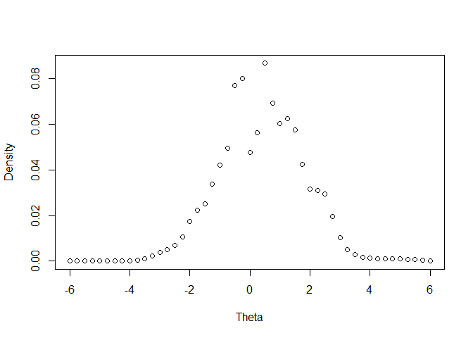
# plot the estimated empirical histogram of latent variable prior distribution
(emphist <- getirt(mod.fix1, what="weights"))
#> theta weight
#> 1 -6.00 2.301252e-10
#> 2 -5.75 1.434595e-09
#> 3 -5.50 8.649281e-09
#> 4 -5.25 5.019868e-08
#> 5 -5.00 2.782912e-07
#> 6 -4.75 1.456751e-06
#> 7 -4.50 7.085630e-06
#> 8 -4.25 3.134808e-05
#> 9 -4.00 1.227012e-04
#> 10 -3.75 4.100603e-04
#> 11 -3.50 1.119742e-03
#> 12 -3.25 2.386354e-03
#> 13 -3.00 3.889321e-03
#> 14 -2.75 5.167720e-03
#> 15 -2.50 6.767224e-03
#> 16 -2.25 1.053445e-02
#> 17 -2.00 1.742567e-02
#> 18 -1.75 2.236173e-02
#> 19 -1.50 2.498735e-02
#> 20 -1.25 3.374293e-02
#> 21 -1.00 4.224442e-02
#> 22 -0.75 4.948939e-02
#> 23 -0.50 7.710828e-02
#> 24 -0.25 8.024288e-02
#> 25 0.00 4.752956e-02
#> 26 0.25 5.636581e-02
#> 27 0.50 8.674316e-02
#> 28 0.75 6.936382e-02
#> 29 1.00 6.035964e-02
#> 30 1.25 6.234864e-02
#> 31 1.50 5.768393e-02
#> 32 1.75 4.254007e-02
#> 33 2.00 3.148380e-02
#> 34 2.25 3.111071e-02
#> 35 2.50 2.935626e-02
#> 36 2.75 1.950494e-02
#> 37 3.00 1.019680e-02
#> 38 3.25 5.154557e-03
#> 39 3.50 2.816466e-03
#> 40 3.75 1.753617e-03
#> 41 4.00 1.282170e-03
#> 42 4.25 1.097172e-03
#> 43 4.50 1.050444e-03
#> 44 4.75 1.046478e-03
#> 45 5.00 1.004637e-03
#> 46 5.25 8.721994e-04
#> 47 5.50 6.557355e-04
#> 48 5.75 4.168380e-04
#> 49 6.00 2.220842e-04
plot(emphist$weight ~ emphist$theta, xlab="Theta", ylab="Density")
##----------------------------------------------------------------------------
# 2. The example code below shows how to prepare the data sets and how to estimate
# the item parameters using Method A:
##----------------------------------------------------------------------------
## Step 1: prepare a data set
## In this example, we generated examinees' true proficiency parameters and simulated
## the item response data using the function "simdat". Because the true
## proficiency parameters are not known in reality, the true proficiencies
## would be replaced with the proficiency estimates for the calibration.
# import the "-prm.txt" output file from flexMIRT
flex_sam <- system.file("extdata", "flexmirt_sample-prm.txt", package = "irtplay")
# select the item meta data
x <- bring.flexmirt(file=flex_sam, "par")$Group1$full_df
# modify the item meta data so that some items follow 1PLM, 2PLM and GPCM
x[c(1:3, 5), 3] <- "1PLM"
x[c(1:3, 5), 4] <- 1
x[c(1:3, 5), 6] <- 0
x[c(4, 8:12), 3] <- "2PLM"
x[c(4, 8:12), 6] <- 0
x[54:55, 3] <- "GPCM"
# generate examinees' abilities from N(0, 1)
set.seed(23)
score <- rnorm(500, mean=0, sd=1)
# simulate the response data
data <- simdat(x=x, theta=score, D=1)
## Step 2: Estimate the item parameters
# 1) item parameter estimation: constrain the slope parameters of the 1PLM to be equal
(mod1 <- est_item(x, data, score, D=1, fix.a.1pl=FALSE, use.gprior=TRUE,
gprior=list(dist="beta", params=c(5, 17)), use.startval=FALSE))
#> Starting...
#> Parsing input...
#> Estimating item parameters...
#> Estimation is finished.
#>
#> Call:
#> est_item(x = x, data = data, score = score, D = 1, fix.a.1pl = FALSE,
#> use.gprior = TRUE, gprior = list(dist = "beta", params = c(5,
#> 17)), use.startval = FALSE)
#>
#> Item calibration using Method-A.
#> All item parameters were successfully converged.
#>
#> Log-likelihood: -15830.66
summary(mod1)
#>
#> Call:
#> est_item(x = x, data = data, score = score, D = 1, fix.a.1pl = FALSE,
#> use.gprior = TRUE, gprior = list(dist = "beta", params = c(5,
#> 17)), use.startval = FALSE)
#>
#> Summary of the Data
#> Number of Items in Response Data: 55
#> Number of Excluded Items: 0
#> Number of free parameters: 162
#> Number of Responses for Each Item:
#> id n
#> 1 CMC1 500
#> 2 CMC2 500
#> 3 CMC3 500
#> 4 CMC4 500
#> 5 CMC5 500
#> 6 CMC6 500
#> 7 CMC7 500
#> 8 CMC8 500
#> 9 CMC9 500
#> 10 CMC10 500
#> 11 CMC11 500
#> 12 CMC12 500
#> 13 CMC13 500
#> 14 CMC14 500
#> 15 CMC15 500
#> 16 CMC16 500
#> 17 CMC17 500
#> 18 CMC18 500
#> 19 CMC19 500
#> 20 CMC20 500
#> 21 CMC21 500
#> 22 CMC22 500
#> 23 CMC23 500
#> 24 CMC24 500
#> 25 CMC25 500
#> 26 CMC26 500
#> 27 CMC27 500
#> 28 CMC28 500
#> 29 CMC29 500
#> 30 CMC30 500
#> 31 CMC31 500
#> 32 CMC32 500
#> 33 CMC33 500
#> 34 CMC34 500
#> 35 CMC35 500
#> 36 CMC36 500
#> 37 CMC37 500
#> 38 CMC38 500
#> 39 CFR1 500
#> 40 CFR2 500
#> 41 AMC1 500
#> 42 AMC2 500
#> 43 AMC3 500
#> 44 AMC4 500
#> 45 AMC5 500
#> 46 AMC6 500
#> 47 AMC7 500
#> 48 AMC8 500
#> 49 AMC9 500
#> 50 AMC10 500
#> 51 AMC11 500
#> 52 AMC12 500
#> 53 AFR1 500
#> 54 AFR2 500
#> 55 AFR3 500
#>
#> Processing time (in seconds)
#> Total computation: 1.36
#>
#> Convergence of Solution
#> All item parameters were successfully converged.
#>
#> Summary of Estimation Results
#> -2loglikelihood: 31661.31
#> Item Parameters:
#> id cats model par.1 se.1 par.2 se.2 par.3 se.3 par.4 se.4
#> 1 CMC1 2 1PLM 1.02 0.06 1.60 0.13 NA NA NA NA
#> 2 CMC2 2 1PLM 1.02 NA -1.06 0.12 NA NA NA NA
#> 3 CMC3 2 1PLM 1.02 NA 0.40 0.10 NA NA NA NA
#> 4 CMC4 2 2PLM 0.96 0.12 -0.43 0.11 NA NA NA NA
#> 5 CMC5 2 1PLM 1.02 NA -0.25 0.10 NA NA NA NA
#> 6 CMC6 2 3PLM 1.88 0.27 0.67 0.09 0.10 0.03 NA NA
#> 7 CMC7 2 3PLM 0.88 0.17 1.03 0.23 0.13 0.05 NA NA
#> 8 CMC8 2 2PLM 0.92 0.12 0.87 0.13 NA NA NA NA
#> 9 CMC9 2 2PLM 1.00 0.12 0.89 0.13 NA NA NA NA
#> 10 CMC10 2 2PLM 1.61 0.15 0.09 0.07 NA NA NA NA
#> 11 CMC11 2 2PLM 1.07 0.12 -0.37 0.10 NA NA NA NA
#> 12 CMC12 2 2PLM 0.94 0.12 1.10 0.15 NA NA NA NA
#> 13 CMC13 2 3PLM 1.35 0.34 1.31 0.17 0.17 0.04 NA NA
#> 14 CMC14 2 3PLM 1.36 0.31 0.15 0.24 0.24 0.08 NA NA
#> 15 CMC15 2 3PLM 1.53 0.27 0.01 0.17 0.20 0.07 NA NA
#> 16 CMC16 2 3PLM 2.10 0.25 0.04 0.08 0.10 0.04 NA NA
#> 17 CMC17 2 3PLM 1.02 0.15 -0.41 0.22 0.16 0.07 NA NA
#> 18 CMC18 2 3PLM 1.27 0.38 1.42 0.20 0.22 0.05 NA NA
#> 19 CMC19 2 3PLM 2.25 0.32 -1.11 0.14 0.17 0.07 NA NA
#> 20 CMC20 2 3PLM 1.47 0.22 -1.74 0.22 0.18 0.08 NA NA
#> 21 CMC21 2 3PLM 1.38 0.21 -1.25 0.23 0.20 0.08 NA NA
#> 22 CMC22 2 3PLM 0.92 0.16 -0.55 0.28 0.19 0.08 NA NA
#> 23 CMC23 2 3PLM 1.10 0.22 -0.12 0.27 0.22 0.09 NA NA
#> 24 CMC24 2 3PLM 1.21 0.34 1.43 0.21 0.22 0.05 NA NA
#> 25 CMC25 2 3PLM 0.83 0.16 -1.51 0.40 0.21 0.09 NA NA
#> 26 CMC26 2 3PLM 1.07 0.18 -2.16 0.35 0.19 0.08 NA NA
#> 27 CMC27 2 3PLM 1.18 0.18 0.09 0.17 0.14 0.06 NA NA
#> 28 CMC28 2 3PLM 2.19 0.31 -0.17 0.11 0.19 0.05 NA NA
#> 29 CMC29 2 3PLM 2.48 0.54 -0.81 0.20 0.38 0.09 NA NA
#> 30 CMC30 2 3PLM 1.88 0.45 0.69 0.15 0.34 0.05 NA NA
#> 31 CMC31 2 3PLM 0.70 0.16 1.00 0.32 0.16 0.07 NA NA
#> 32 CMC32 2 3PLM 1.73 0.30 -0.78 0.21 0.26 0.09 NA NA
#> 33 CMC33 2 3PLM 1.07 0.17 -1.45 0.28 0.19 0.08 NA NA
#> 34 CMC34 2 3PLM 1.04 0.17 0.21 0.20 0.16 0.06 NA NA
#> 35 CMC35 2 3PLM 1.36 0.19 -0.45 0.17 0.16 0.06 NA NA
#> 36 CMC36 2 3PLM 0.88 0.17 0.97 0.23 0.14 0.05 NA NA
#> 37 CMC37 2 3PLM 2.13 0.26 -0.25 0.09 0.13 0.05 NA NA
#> 38 CMC38 2 3PLM 0.87 0.17 -0.31 0.32 0.20 0.09 NA NA
#> 39 CFR1 5 GRM 2.00 0.14 -1.88 0.12 -1.25 0.08 -0.70 0.06
#> 40 CFR2 5 GRM 1.39 0.11 -0.80 0.09 -0.13 0.07 0.60 0.08
#> 41 AMC1 2 3PLM 1.81 0.39 0.74 0.14 0.28 0.05 NA NA
#> 42 AMC2 2 3PLM 1.70 0.25 -1.59 0.20 0.19 0.08 NA NA
#> 43 AMC3 2 3PLM 1.30 0.25 0.68 0.16 0.16 0.05 NA NA
#> 44 AMC4 2 3PLM 0.94 0.17 -0.18 0.26 0.18 0.07 NA NA
#> 45 AMC5 2 3PLM 1.69 0.65 2.11 0.26 0.19 0.03 NA NA
#> 46 AMC6 2 3PLM 2.83 0.64 1.44 0.10 0.15 0.02 NA NA
#> 47 AMC7 2 3PLM 1.69 0.41 0.37 0.18 0.25 0.07 NA NA
#> 48 AMC8 2 3PLM 1.65 0.29 0.39 0.14 0.20 0.05 NA NA
#> 49 AMC9 2 3PLM 1.55 0.26 0.49 0.13 0.15 0.05 NA NA
#> 50 AMC10 2 3PLM 2.48 0.51 1.31 0.10 0.13 0.02 NA NA
#> 51 AMC11 2 3PLM 1.73 0.23 -1.02 0.15 0.16 0.07 NA NA
#> 52 AMC12 2 3PLM 0.95 0.20 -0.83 0.38 0.24 0.10 NA NA
#> 53 AFR1 5 GRM 1.14 0.10 -0.30 0.09 0.30 0.09 0.92 0.11
#> 54 AFR2 5 GPCM 1.33 0.11 -1.99 0.21 -1.31 0.15 -0.72 0.12
#> 55 AFR3 5 GPCM 0.89 0.07 -0.80 0.15 0.15 0.15 0.46 0.16
#> par.5 se.5
#> 1 NA NA
#> 2 NA NA
#> 3 NA NA
#> 4 NA NA
#> 5 NA NA
#> 6 NA NA
#> 7 NA NA
#> 8 NA NA
#> 9 NA NA
#> 10 NA NA
#> 11 NA NA
#> 12 NA NA
#> 13 NA NA
#> 14 NA NA
#> 15 NA NA
#> 16 NA NA
#> 17 NA NA
#> 18 NA NA
#> 19 NA NA
#> 20 NA NA
#> 21 NA NA
#> 22 NA NA
#> 23 NA NA
#> 24 NA NA
#> 25 NA NA
#> 26 NA NA
#> 27 NA NA
#> 28 NA NA
#> 29 NA NA
#> 30 NA NA
#> 31 NA NA
#> 32 NA NA
#> 33 NA NA
#> 34 NA NA
#> 35 NA NA
#> 36 NA NA
#> 37 NA NA
#> 38 NA NA
#> 39 -0.23 0.06
#> 40 1.09 0.10
#> 41 NA NA
#> 42 NA NA
#> 43 NA NA
#> 44 NA NA
#> 45 NA NA
#> 46 NA NA
#> 47 NA NA
#> 48 NA NA
#> 49 NA NA
#> 50 NA NA
#> 51 NA NA
#> 52 NA NA
#> 53 1.35 0.13
#> 54 -0.21 0.10
#> 55 1.35 0.19
#>
#> Group Parameters:
#> mu sigma
#> 0.03 1.02
# 2) item parameter estimation: fix the slope parameters of the 1PLM to 1
(mod2 <- est_item(x, data, score, D=1, fix.a.1pl=TRUE, a.val.1pl=1, use.gprior=TRUE,
gprior=list(dist="beta", params=c(5, 17)), use.startval=FALSE))
#> Starting...
#> Parsing input...
#> Estimating item parameters...
#> Estimation is finished.
#>
#> Call:
#> est_item(x = x, data = data, score = score, D = 1, fix.a.1pl = TRUE,
#> a.val.1pl = 1, use.gprior = TRUE, gprior = list(dist = "beta",
#> params = c(5, 17)), use.startval = FALSE)
#>
#> Item calibration using Method-A.
#> All item parameters were successfully converged.
#>
#> Log-likelihood: -15830.7
summary(mod2)
#>
#> Call:
#> est_item(x = x, data = data, score = score, D = 1, fix.a.1pl = TRUE,
#> a.val.1pl = 1, use.gprior = TRUE, gprior = list(dist = "beta",
#> params = c(5, 17)), use.startval = FALSE)
#>
#> Summary of the Data
#> Number of Items in Response Data: 55
#> Number of Excluded Items: 0
#> Number of free parameters: 161
#> Number of Responses for Each Item:
#> id n
#> 1 CMC1 500
#> 2 CMC2 500
#> 3 CMC3 500
#> 4 CMC4 500
#> 5 CMC5 500
#> 6 CMC6 500
#> 7 CMC7 500
#> 8 CMC8 500
#> 9 CMC9 500
#> 10 CMC10 500
#> 11 CMC11 500
#> 12 CMC12 500
#> 13 CMC13 500
#> 14 CMC14 500
#> 15 CMC15 500
#> 16 CMC16 500
#> 17 CMC17 500
#> 18 CMC18 500
#> 19 CMC19 500
#> 20 CMC20 500
#> 21 CMC21 500
#> 22 CMC22 500
#> 23 CMC23 500
#> 24 CMC24 500
#> 25 CMC25 500
#> 26 CMC26 500
#> 27 CMC27 500
#> 28 CMC28 500
#> 29 CMC29 500
#> 30 CMC30 500
#> 31 CMC31 500
#> 32 CMC32 500
#> 33 CMC33 500
#> 34 CMC34 500
#> 35 CMC35 500
#> 36 CMC36 500
#> 37 CMC37 500
#> 38 CMC38 500
#> 39 CFR1 500
#> 40 CFR2 500
#> 41 AMC1 500
#> 42 AMC2 500
#> 43 AMC3 500
#> 44 AMC4 500
#> 45 AMC5 500
#> 46 AMC6 500
#> 47 AMC7 500
#> 48 AMC8 500
#> 49 AMC9 500
#> 50 AMC10 500
#> 51 AMC11 500
#> 52 AMC12 500
#> 53 AFR1 500
#> 54 AFR2 500
#> 55 AFR3 500
#>
#> Processing time (in seconds)
#> Total computation: 2.05
#>
#> Convergence of Solution
#> All item parameters were successfully converged.
#>
#> Summary of Estimation Results
#> -2loglikelihood: 31661.4
#> Item Parameters:
#> id cats model par.1 se.1 par.2 se.2 par.3 se.3 par.4 se.4
#> 1 CMC1 2 1PLM 1.00 NA 1.62 0.12 NA NA NA NA
#> 2 CMC2 2 1PLM 1.00 NA -1.08 0.11 NA NA NA NA
#> 3 CMC3 2 1PLM 1.00 NA 0.40 0.10 NA NA NA NA
#> 4 CMC4 2 2PLM 0.96 0.12 -0.43 0.11 NA NA NA NA
#> 5 CMC5 2 1PLM 1.00 NA -0.25 0.10 NA NA NA NA
#> 6 CMC6 2 3PLM 1.88 0.27 0.67 0.09 0.10 0.03 NA NA
#> 7 CMC7 2 3PLM 0.88 0.17 1.03 0.23 0.13 0.05 NA NA
#> 8 CMC8 2 2PLM 0.92 0.12 0.87 0.13 NA NA NA NA
#> 9 CMC9 2 2PLM 1.00 0.12 0.89 0.13 NA NA NA NA
#> 10 CMC10 2 2PLM 1.61 0.15 0.09 0.07 NA NA NA NA
#> 11 CMC11 2 2PLM 1.07 0.12 -0.37 0.10 NA NA NA NA
#> 12 CMC12 2 2PLM 0.94 0.12 1.10 0.15 NA NA NA NA
#> 13 CMC13 2 3PLM 1.35 0.34 1.31 0.17 0.17 0.04 NA NA
#> 14 CMC14 2 3PLM 1.36 0.31 0.15 0.24 0.24 0.08 NA NA
#> 15 CMC15 2 3PLM 1.53 0.27 0.01 0.17 0.20 0.07 NA NA
#> 16 CMC16 2 3PLM 2.10 0.25 0.04 0.08 0.10 0.04 NA NA
#> 17 CMC17 2 3PLM 1.02 0.15 -0.41 0.22 0.16 0.07 NA NA
#> 18 CMC18 2 3PLM 1.27 0.38 1.42 0.20 0.22 0.05 NA NA
#> 19 CMC19 2 3PLM 2.25 0.32 -1.11 0.14 0.17 0.07 NA NA
#> 20 CMC20 2 3PLM 1.47 0.22 -1.74 0.22 0.18 0.08 NA NA
#> 21 CMC21 2 3PLM 1.38 0.21 -1.25 0.23 0.20 0.08 NA NA
#> 22 CMC22 2 3PLM 0.92 0.16 -0.55 0.28 0.19 0.08 NA NA
#> 23 CMC23 2 3PLM 1.10 0.22 -0.12 0.27 0.22 0.09 NA NA
#> 24 CMC24 2 3PLM 1.21 0.34 1.43 0.21 0.22 0.05 NA NA
#> 25 CMC25 2 3PLM 0.83 0.16 -1.51 0.40 0.21 0.09 NA NA
#> 26 CMC26 2 3PLM 1.07 0.18 -2.16 0.35 0.19 0.08 NA NA
#> 27 CMC27 2 3PLM 1.18 0.18 0.09 0.17 0.14 0.06 NA NA
#> 28 CMC28 2 3PLM 2.19 0.31 -0.17 0.11 0.19 0.05 NA NA
#> 29 CMC29 2 3PLM 2.48 0.54 -0.81 0.20 0.38 0.09 NA NA
#> 30 CMC30 2 3PLM 1.88 0.45 0.69 0.15 0.34 0.05 NA NA
#> 31 CMC31 2 3PLM 0.70 0.16 1.00 0.32 0.16 0.07 NA NA
#> 32 CMC32 2 3PLM 1.73 0.30 -0.78 0.21 0.26 0.09 NA NA
#> 33 CMC33 2 3PLM 1.07 0.17 -1.45 0.28 0.19 0.08 NA NA
#> 34 CMC34 2 3PLM 1.04 0.17 0.21 0.20 0.16 0.06 NA NA
#> 35 CMC35 2 3PLM 1.36 0.19 -0.45 0.17 0.16 0.06 NA NA
#> 36 CMC36 2 3PLM 0.88 0.17 0.97 0.23 0.14 0.05 NA NA
#> 37 CMC37 2 3PLM 2.13 0.26 -0.25 0.09 0.13 0.05 NA NA
#> 38 CMC38 2 3PLM 0.87 0.17 -0.31 0.32 0.20 0.09 NA NA
#> 39 CFR1 5 GRM 2.00 0.14 -1.88 0.12 -1.25 0.08 -0.70 0.06
#> 40 CFR2 5 GRM 1.39 0.11 -0.80 0.09 -0.13 0.07 0.60 0.08
#> 41 AMC1 2 3PLM 1.81 0.39 0.74 0.14 0.28 0.05 NA NA
#> 42 AMC2 2 3PLM 1.70 0.25 -1.59 0.20 0.19 0.08 NA NA
#> 43 AMC3 2 3PLM 1.30 0.25 0.68 0.16 0.16 0.05 NA NA
#> 44 AMC4 2 3PLM 0.94 0.17 -0.18 0.26 0.18 0.07 NA NA
#> 45 AMC5 2 3PLM 1.69 0.65 2.11 0.26 0.19 0.03 NA NA
#> 46 AMC6 2 3PLM 2.83 0.64 1.44 0.10 0.15 0.02 NA NA
#> 47 AMC7 2 3PLM 1.69 0.41 0.37 0.18 0.25 0.07 NA NA
#> 48 AMC8 2 3PLM 1.65 0.29 0.39 0.14 0.20 0.05 NA NA
#> 49 AMC9 2 3PLM 1.55 0.26 0.49 0.13 0.15 0.05 NA NA
#> 50 AMC10 2 3PLM 2.48 0.51 1.31 0.10 0.13 0.02 NA NA
#> 51 AMC11 2 3PLM 1.73 0.23 -1.02 0.15 0.16 0.07 NA NA
#> 52 AMC12 2 3PLM 0.95 0.20 -0.83 0.38 0.24 0.10 NA NA
#> 53 AFR1 5 GRM 1.14 0.10 -0.30 0.09 0.30 0.09 0.92 0.11
#> 54 AFR2 5 GPCM 1.33 0.11 -1.99 0.21 -1.31 0.15 -0.72 0.12
#> 55 AFR3 5 GPCM 0.89 0.07 -0.80 0.15 0.15 0.15 0.46 0.16
#> par.5 se.5
#> 1 NA NA
#> 2 NA NA
#> 3 NA NA
#> 4 NA NA
#> 5 NA NA
#> 6 NA NA
#> 7 NA NA
#> 8 NA NA
#> 9 NA NA
#> 10 NA NA
#> 11 NA NA
#> 12 NA NA
#> 13 NA NA
#> 14 NA NA
#> 15 NA NA
#> 16 NA NA
#> 17 NA NA
#> 18 NA NA
#> 19 NA NA
#> 20 NA NA
#> 21 NA NA
#> 22 NA NA
#> 23 NA NA
#> 24 NA NA
#> 25 NA NA
#> 26 NA NA
#> 27 NA NA
#> 28 NA NA
#> 29 NA NA
#> 30 NA NA
#> 31 NA NA
#> 32 NA NA
#> 33 NA NA
#> 34 NA NA
#> 35 NA NA
#> 36 NA NA
#> 37 NA NA
#> 38 NA NA
#> 39 -0.23 0.06
#> 40 1.09 0.10
#> 41 NA NA
#> 42 NA NA
#> 43 NA NA
#> 44 NA NA
#> 45 NA NA
#> 46 NA NA
#> 47 NA NA
#> 48 NA NA
#> 49 NA NA
#> 50 NA NA
#> 51 NA NA
#> 52 NA NA
#> 53 1.35 0.13
#> 54 -0.21 0.10
#> 55 1.35 0.19
#>
#> Group Parameters:
#> mu sigma
#> 0.03 1.02
# 3) item parameter estimation: fix the guessing parameters of the 3PLM to 0.2
(mod3 <- est_item(x, data, score, D=1, fix.a.1pl=TRUE, fix.g=TRUE, a.val.1pl=1, g.val=.2,
use.startval=FALSE))
#> Starting...
#> Parsing input...
#> Estimating item parameters...
#> Estimation is finished.
#>
#> Call:
#> est_item(x = x, data = data, score = score, D = 1, fix.a.1pl = TRUE,
#> fix.g = TRUE, a.val.1pl = 1, g.val = 0.2, use.startval = FALSE)
#>
#> Item calibration using Method-A.
#> All item parameters were successfully converged.
#>
#> Log-likelihood: -15916.26
summary(mod3)
#>
#> Call:
#> est_item(x = x, data = data, score = score, D = 1, fix.a.1pl = TRUE,
#> fix.g = TRUE, a.val.1pl = 1, g.val = 0.2, use.startval = FALSE)
#>
#> Summary of the Data
#> Number of Items in Response Data: 55
#> Number of Excluded Items: 0
#> Number of free parameters: 121
#> Number of Responses for Each Item:
#> id n
#> 1 CMC1 500
#> 2 CMC2 500
#> 3 CMC3 500
#> 4 CMC4 500
#> 5 CMC5 500
#> 6 CMC6 500
#> 7 CMC7 500
#> 8 CMC8 500
#> 9 CMC9 500
#> 10 CMC10 500
#> 11 CMC11 500
#> 12 CMC12 500
#> 13 CMC13 500
#> 14 CMC14 500
#> 15 CMC15 500
#> 16 CMC16 500
#> 17 CMC17 500
#> 18 CMC18 500
#> 19 CMC19 500
#> 20 CMC20 500
#> 21 CMC21 500
#> 22 CMC22 500
#> 23 CMC23 500
#> 24 CMC24 500
#> 25 CMC25 500
#> 26 CMC26 500
#> 27 CMC27 500
#> 28 CMC28 500
#> 29 CMC29 500
#> 30 CMC30 500
#> 31 CMC31 500
#> 32 CMC32 500
#> 33 CMC33 500
#> 34 CMC34 500
#> 35 CMC35 500
#> 36 CMC36 500
#> 37 CMC37 500
#> 38 CMC38 500
#> 39 CFR1 500
#> 40 CFR2 500
#> 41 AMC1 500
#> 42 AMC2 500
#> 43 AMC3 500
#> 44 AMC4 500
#> 45 AMC5 500
#> 46 AMC6 500
#> 47 AMC7 500
#> 48 AMC8 500
#> 49 AMC9 500
#> 50 AMC10 500
#> 51 AMC11 500
#> 52 AMC12 500
#> 53 AFR1 500
#> 54 AFR2 500
#> 55 AFR3 500
#>
#> Processing time (in seconds)
#> Total computation: 1.18
#>
#> Convergence of Solution
#> All item parameters were successfully converged.
#>
#> Summary of Estimation Results
#> -2loglikelihood: 31832.52
#> Item Parameters:
#> id cats model par.1 se.1 par.2 se.2 par.3 se.3 par.4 se.4
#> 1 CMC1 2 1PLM 1.00 NA 1.62 0.12 NA NA NA NA
#> 2 CMC2 2 1PLM 1.00 NA -1.08 0.11 NA NA NA NA
#> 3 CMC3 2 1PLM 1.00 NA 0.40 0.10 NA NA NA NA
#> 4 CMC4 2 2PLM 0.96 0.12 -0.43 0.11 NA NA NA NA
#> 5 CMC5 2 1PLM 1.00 NA -0.25 0.10 NA NA NA NA
#> 6 CMC6 2 3PLM 2.25 0.29 0.83 0.08 0.20 NA NA NA
#> 7 CMC7 2 3PLM 1.00 0.17 1.22 0.19 0.20 NA NA NA
#> 8 CMC8 2 2PLM 0.92 0.12 0.87 0.13 NA NA NA NA
#> 9 CMC9 2 2PLM 1.00 0.12 0.89 0.13 NA NA NA NA
#> 10 CMC10 2 2PLM 1.61 0.15 0.09 0.07 NA NA NA NA
#> 11 CMC11 2 2PLM 1.07 0.12 -0.37 0.10 NA NA NA NA
#> 12 CMC12 2 2PLM 0.94 0.12 1.10 0.15 NA NA NA NA
#> 13 CMC13 2 3PLM 1.53 0.28 1.37 0.15 0.20 NA NA NA
#> 14 CMC14 2 3PLM 1.26 0.18 0.05 0.10 0.20 NA NA NA
#> 15 CMC15 2 3PLM 1.52 0.20 0.00 0.09 0.20 NA NA NA
#> 16 CMC16 2 3PLM 2.36 0.27 0.18 0.07 0.20 NA NA NA
#> 17 CMC17 2 3PLM 1.06 0.15 -0.30 0.12 0.20 NA NA NA
#> 18 CMC18 2 3PLM 1.16 0.23 1.38 0.19 0.20 NA NA NA
#> 19 CMC19 2 3PLM 2.30 0.30 -1.07 0.10 0.20 NA NA NA
#> 20 CMC20 2 3PLM 1.48 0.22 -1.71 0.19 0.20 NA NA NA
#> 21 CMC21 2 3PLM 1.38 0.19 -1.25 0.16 0.20 NA NA NA
#> 22 CMC22 2 3PLM 0.93 0.14 -0.52 0.15 0.20 NA NA NA
#> 23 CMC23 2 3PLM 1.08 0.16 -0.17 0.12 0.20 NA NA NA
#> 24 CMC24 2 3PLM 1.13 0.23 1.40 0.19 0.20 NA NA NA
#> 25 CMC25 2 3PLM 0.82 0.15 -1.55 0.28 0.20 NA NA NA
#> 26 CMC26 2 3PLM 1.07 0.18 -2.14 0.31 0.20 NA NA NA
#> 27 CMC27 2 3PLM 1.27 0.17 0.22 0.10 0.20 NA NA NA
#> 28 CMC28 2 3PLM 2.22 0.27 -0.15 0.07 0.20 NA NA NA
#> 29 CMC29 2 3PLM 1.84 0.28 -1.19 0.14 0.20 NA NA NA
#> 30 CMC30 2 3PLM 1.19 0.20 0.35 0.11 0.20 NA NA NA
#> 31 CMC31 2 3PLM 0.76 0.15 1.15 0.23 0.20 NA NA NA
#> 32 CMC32 2 3PLM 1.62 0.22 -0.90 0.12 0.20 NA NA NA
#> 33 CMC33 2 3PLM 1.07 0.16 -1.43 0.21 0.20 NA NA NA
#> 34 CMC34 2 3PLM 1.11 0.16 0.33 0.12 0.20 NA NA NA
#> 35 CMC35 2 3PLM 1.42 0.18 -0.36 0.10 0.20 NA NA NA
#> 36 CMC36 2 3PLM 1.00 0.17 1.15 0.18 0.20 NA NA NA
#> 37 CMC37 2 3PLM 2.30 0.27 -0.15 0.07 0.20 NA NA NA
#> 38 CMC38 2 3PLM 0.87 0.14 -0.33 0.15 0.20 NA NA NA
#> 39 CFR1 5 GRM 2.00 0.14 -1.88 0.12 -1.25 0.08 -0.70 0.06
#> 40 CFR2 5 GRM 1.39 0.11 -0.80 0.09 -0.13 0.07 0.60 0.08
#> 41 AMC1 2 3PLM 1.45 0.22 0.57 0.10 0.20 NA NA NA
#> 42 AMC2 2 3PLM 1.72 0.25 -1.57 0.16 0.20 NA NA NA
#> 43 AMC3 2 3PLM 1.44 0.21 0.77 0.11 0.20 NA NA NA
#> 44 AMC4 2 3PLM 0.96 0.15 -0.13 0.13 0.20 NA NA NA
#> 45 AMC5 2 3PLM 1.83 0.53 2.10 0.25 0.20 NA NA NA
#> 46 AMC6 2 3PLM 3.32 0.68 1.50 0.09 0.20 NA NA NA
#> 47 AMC7 2 3PLM 1.48 0.21 0.25 0.09 0.20 NA NA NA
#> 48 AMC8 2 3PLM 1.65 0.23 0.39 0.09 0.20 NA NA NA
#> 49 AMC9 2 3PLM 1.72 0.23 0.59 0.09 0.20 NA NA NA
#> 50 AMC10 2 3PLM 3.21 0.62 1.40 0.09 0.20 NA NA NA
#> 51 AMC11 2 3PLM 1.78 0.22 -0.96 0.11 0.20 NA NA NA
#> 52 AMC12 2 3PLM 0.91 0.15 -0.96 0.19 0.20 NA NA NA
#> 53 AFR1 5 GRM 1.14 0.10 -0.30 0.09 0.30 0.09 0.92 0.11
#> 54 AFR2 5 GPCM 1.33 0.11 -1.99 0.21 -1.31 0.15 -0.72 0.12
#> 55 AFR3 5 GPCM 0.89 0.07 -0.80 0.15 0.15 0.15 0.46 0.16
#> par.5 se.5
#> 1 NA NA
#> 2 NA NA
#> 3 NA NA
#> 4 NA NA
#> 5 NA NA
#> 6 NA NA
#> 7 NA NA
#> 8 NA NA
#> 9 NA NA
#> 10 NA NA
#> 11 NA NA
#> 12 NA NA
#> 13 NA NA
#> 14 NA NA
#> 15 NA NA
#> 16 NA NA
#> 17 NA NA
#> 18 NA NA
#> 19 NA NA
#> 20 NA NA
#> 21 NA NA
#> 22 NA NA
#> 23 NA NA
#> 24 NA NA
#> 25 NA NA
#> 26 NA NA
#> 27 NA NA
#> 28 NA NA
#> 29 NA NA
#> 30 NA NA
#> 31 NA NA
#> 32 NA NA
#> 33 NA NA
#> 34 NA NA
#> 35 NA NA
#> 36 NA NA
#> 37 NA NA
#> 38 NA NA
#> 39 -0.23 0.06
#> 40 1.09 0.10
#> 41 NA NA
#> 42 NA NA
#> 43 NA NA
#> 44 NA NA
#> 45 NA NA
#> 46 NA NA
#> 47 NA NA
#> 48 NA NA
#> 49 NA NA
#> 50 NA NA
#> 51 NA NA
#> 52 NA NA
#> 53 1.35 0.13
#> 54 -0.21 0.10
#> 55 1.35 0.19
#>
#> Group Parameters:
#> mu sigma
#> 0.03 1.02
##----------------------------------------------------------------------------
# 3. The example code below shows how to prepare the data sets and how to conduct
# the IRT model-data fit analysis:
##----------------------------------------------------------------------------
## Step 1: prepare a data set for IRT
## In this example, we use the simulated mixed-item format CAT Data
## But, only items that have item responses more than 1,000 are assessed.
# find the location of items that have more than 1,000 item responses
over1000 <- which(colSums(simCAT_MX$res.dat, na.rm=TRUE) > 1000)
# (1) item meta data
x <- simCAT_MX$item.prm[over1000, ]
dim(x)
#> [1] 113 7
print(x[1:10, ])
#> id cats model par.1 par.2 par.3 par.4
#> 2 V2 2 2PLM 0.9152754 1.3843593 NA NA
#> 3 V3 2 2PLM 1.3454796 -1.2554919 NA NA
#> 5 V5 2 2PLM 1.0862914 1.7114409 NA NA
#> 6 V6 2 2PLM 1.1311496 -0.6029080 NA NA
#> 7 V7 2 2PLM 1.2012407 -0.4721664 NA NA
#> 8 V8 2 2PLM 1.3244155 -0.6353713 NA NA
#> 10 V10 2 2PLM 1.2487125 0.1381082 NA NA
#> 11 V11 2 2PLM 1.4413208 1.2276303 NA NA
#> 12 V12 2 2PLM 1.2077273 -0.8017795 NA NA
#> 13 V13 2 2PLM 1.1715456 -1.0803926 NA NA
# (2) examinee's ability estimates
score <- simCAT_MX$score
length(score)
#> [1] 30000
print(score[1:100])
#> [1] -0.30311440 -0.67224807 -0.73474583 1.76935738 -0.91017203 -0.28448278
#> [7] 0.81656431 -1.66434615 0.59312008 -0.35182937 0.23129679 -0.93107524
#> [13] -0.29971993 -0.32700449 -0.22271651 1.48912121 -0.92927809 0.43453041
#> [19] -0.01795450 -0.28365286 0.01115173 -0.76101441 0.12144273 0.83096135
#> [25] 1.96600585 -0.83510402 -0.40268865 -0.05605526 0.72398446 -0.16026059
#> [31] -1.09011778 1.22126764 -0.13340360 -1.28230720 -1.05581980 0.83484173
#> [37] -0.52136360 -0.66913590 -1.08580804 1.73214834 0.56950387 0.48016332
#> [43] -0.03472720 -2.17577824 0.44127032 0.98913071 1.43861714 -1.08133809
#> [49] -0.69016072 0.19325797 0.89998383 1.25383167 -1.09600809 0.50519143
#> [55] -0.51707395 -0.39474484 -0.45031102 1.85675021 1.50768131 1.06011811
#> [61] -0.41064797 1.10960278 -0.68853387 -0.59397660 -0.65326436 0.29147751
#> [67] -1.86787473 1.04838050 -1.14582092 1.07395234 -0.03828693 0.08445559
#> [73] 0.34582524 0.72300905 0.84448992 -1.86488055 0.77121937 1.66573208
#> [79] 0.10311673 -0.50768866 -1.60992457 -0.23074682 0.16162326 0.26091160
#> [85] 0.60682182 0.65415304 -0.69923141 1.07545766 0.24060267 -0.93542383
#> [91] 1.24988766 -0.01826940 1.27403936 0.10985621 -1.19092047 0.79614598
#> [97] 0.62302338 -0.89455596 -0.03472720 0.20250837
# (3) response data
data <- simCAT_MX$res.dat[, over1000]
dim(data)
#> [1] 30000 113
print(data[1:20, 1:6])
#> Item.dc.2 Item.dc.3 Item.dc.5 Item.dc.6 Item.dc.7 Item.dc.8
#> [1,] NA NA NA NA 0 1
#> [2,] NA NA NA NA 0 1
#> [3,] NA NA NA NA 1 1
#> [4,] NA NA 0 NA NA NA
#> [5,] NA 1 NA 0 1 1
#> [6,] NA 0 NA 0 1 0
#> [7,] NA NA NA NA NA NA
#> [8,] NA 1 NA 1 1 0
#> [9,] NA NA 0 NA NA NA
#> [10,] NA 0 NA 1 1 0
#> [11,] NA NA 0 NA NA NA
#> [12,] NA 1 NA 0 1 1
#> [13,] NA 0 NA 1 1 0
#> [14,] NA NA NA NA 1 NA
#> [15,] NA NA NA 1 1 1
#> [16,] 1 NA 0 NA NA NA
#> [17,] NA 0 NA 0 1 0
#> [18,] NA NA NA NA NA NA
#> [19,] NA 0 NA 0 1 1
#> [20,] NA NA NA NA NA NA
## Step 2: Compute the IRT mode-data fit statistics
# (1) the use of "equal.width"
fit1 <- irtfit(x=x, score=score, data=data, group.method="equal.width",
n.width=11, loc.theta="average", range.score=c(-4, 4), D=1, alpha=0.05,
missing=NA, overSR = 2.5)
# what kinds of internal objects does the results have?
names(fit1)
#> [1] "fit_stat" "contingency.fitstat" "contingency.plot"
#> [4] "item_df" "individual.info" "ancillary"
#> [7] "call"
# show the results of the fit statistics
fit1$fit_stat[1:10, ]
#> id X2 G2 df.X2 df.G2 crit.value.X2 crit.value.G2 p.value.X2
#> 1 V2 75.070 75.209 8 10 15.51 18.31 0
#> 2 V3 186.880 168.082 8 10 15.51 18.31 0
#> 3 V5 151.329 139.213 8 10 15.51 18.31 0
#> 4 V6 178.409 157.911 8 10 15.51 18.31 0
#> 5 V7 185.438 170.360 9 11 16.92 19.68 0
#> 6 V8 209.653 193.001 8 10 15.51 18.31 0
#> 7 V10 267.444 239.563 9 11 16.92 19.68 0
#> 8 V11 148.896 133.209 7 9 14.07 16.92 0
#> 9 V12 139.295 125.647 9 11 16.92 19.68 0
#> 10 V13 128.422 117.439 9 11 16.92 19.68 0
#> p.value.G2 outfit infit N overSR.prop
#> 1 0 1.018 1.016 2018 0.364
#> 2 0 1.124 1.090 11041 0.636
#> 3 0 1.133 1.111 5181 0.727
#> 4 0 1.056 1.045 13599 0.545
#> 5 0 1.078 1.059 18293 0.455
#> 6 0 1.098 1.075 16163 0.636
#> 7 0 1.097 1.073 19702 0.727
#> 8 0 1.129 1.083 13885 0.455
#> 9 0 1.065 1.051 12118 0.636
#> 10 0 1.075 1.059 10719 0.545
# show the contingency tables for the first item (dichotomous)
fit1$contingency.fitstat[[1]]
#> N freq.0 freq.1 obs.prop.0 obs.prop.1 exp.prob.0 exp.prob.1 raw_resid.0
#> 1 8 5 3 0.6250000 0.3750000 0.7627914 0.2372086 -0.13779141
#> 2 14 8 6 0.5714286 0.4285714 0.7121079 0.2878921 -0.14067932
#> 3 60 34 26 0.5666667 0.4333333 0.6708959 0.3291041 -0.10422928
#> 4 185 99 86 0.5351351 0.4648649 0.6230537 0.3769463 -0.08791853
#> 5 240 115 125 0.4791667 0.5208333 0.5765337 0.4234663 -0.09736699
#> 6 349 145 204 0.4154728 0.5845272 0.5301760 0.4698240 -0.11470327
#> 7 325 114 211 0.3507692 0.6492308 0.4784096 0.5215904 -0.12764036
#> 8 246 82 164 0.3333333 0.6666667 0.4419993 0.5580007 -0.10866594
#> 9 377 139 238 0.3687003 0.6312997 0.4086532 0.5913468 -0.03995295
#> 10 214 78 136 0.3644860 0.6355140 0.3394647 0.6605353 0.02502128
#> raw_resid.1
#> 1 0.13779141
#> 2 0.14067932
#> 3 0.10422928
#> 4 0.08791853
#> 5 0.09736699
#> 6 0.11470327
#> 7 0.12764036
#> 8 0.10866594
#> 9 0.03995295
#> 10 -0.02502128
# (2) the use of "equal.freq"
fit2 <- irtfit(x=x, score=score, data=data, group.method="equal.freq",
n.width=11, loc.theta="average", range.score=c(-4, 4), D=1, alpha=0.05,
missing=NA)
# show the results of the fit statistics
fit2$fit_stat[1:10, ]
#> id X2 G2 df.X2 df.G2 crit.value.X2 crit.value.G2 p.value.X2
#> 1 V2 77.967 78.144 9 11 16.92 19.68 0
#> 2 V3 202.035 181.832 9 11 16.92 19.68 0
#> 3 V5 146.383 135.908 9 11 16.92 19.68 0
#> 4 V6 140.038 133.287 9 11 16.92 19.68 0
#> 5 V7 188.814 177.526 9 11 16.92 19.68 0
#> 6 V8 211.279 196.328 9 11 16.92 19.68 0
#> 7 V10 259.669 239.292 9 11 16.92 19.68 0
#> 8 V11 166.427 150.419 9 11 16.92 19.68 0
#> 9 V12 145.789 134.690 9 11 16.92 19.68 0
#> 10 V13 141.283 132.270 9 11 16.92 19.68 0
#> p.value.G2 outfit infit N overSR.prop
#> 1 0 1.018 1.016 2018 0.727
#> 2 0 1.124 1.090 11041 0.636
#> 3 0 1.133 1.111 5181 0.727
#> 4 0 1.056 1.045 13599 0.545
#> 5 0 1.078 1.059 18293 0.455
#> 6 0 1.098 1.075 16163 0.545
#> 7 0 1.097 1.073 19702 0.636
#> 8 0 1.129 1.083 13885 0.636
#> 9 0 1.065 1.051 12118 0.364
#> 10 0 1.075 1.059 10719 0.636
# show the contingency table for the fourth item (polytomous)
fit2$contingency.fitstat[[4]]
#> N freq.0 freq.1 obs.prop.0 obs.prop.1 exp.prob.0 exp.prob.1 raw_resid.0
#> 1 1241 967 274 0.7792103 0.2207897 0.8038510 0.1961490 -0.024640641
#> 2 1243 879 364 0.7071601 0.2928399 0.7161793 0.2838207 -0.009019180
#> 3 1243 784 459 0.6307321 0.3692679 0.6575849 0.3424151 -0.026852795
#> 4 1219 747 472 0.6127974 0.3872026 0.6049393 0.3950607 0.007858099
#> 5 1236 705 531 0.5703883 0.4296117 0.5613454 0.4386546 0.009042942
#> 6 1243 677 566 0.5446500 0.4553500 0.5279560 0.4720440 0.016694048
#> 7 1270 662 608 0.5212598 0.4787402 0.4925592 0.5074408 0.028700633
#> 8 1230 616 614 0.5008130 0.4991870 0.4491759 0.5508241 0.051637085
#> 9 1207 553 654 0.4581607 0.5418393 0.4027790 0.5972210 0.055381721
#> 10 1233 494 739 0.4006488 0.5993512 0.3509261 0.6490739 0.049722759
#> 11 1234 465 769 0.3768233 0.6231767 0.2630181 0.7369819 0.113805214
#> raw_resid.1
#> 1 0.024640641
#> 2 0.009019180
#> 3 0.026852795
#> 4 -0.007858099
#> 5 -0.009042942
#> 6 -0.016694048
#> 7 -0.028700633
#> 8 -0.051637085
#> 9 -0.055381721
#> 10 -0.049722759
#> 11 -0.113805214
## Step 3: Draw the IRT residual plots
# 1. the dichotomous item
# (1) both raw and standardized residual plots using the object "fit1"
plot(x=fit1, item.loc=1, type = "both", ci.method = "wald", ylim.sr.adjust=TRUE)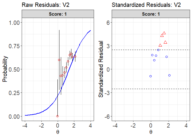
#>                               theta   N freq.0 freq.1 obs.prop.0 obs.prop.1
#> [-0.1218815,0.08512996] -0.02529272   3      3      0  1.0000000  0.0000000
#> (0.08512996,0.2921415]   0.18431014   5      2      3  0.4000000  0.6000000
#> (0.2921415,0.499153]     0.39488272  14      8      6  0.5714286  0.4285714
#> (0.499153,0.7061645]     0.60618911  60     34     26  0.5666667  0.4333333
#> (0.7061645,0.913176]     0.83531169 185     99     86  0.5351351  0.4648649
#> (0.913176,1.120187]      1.04723712 240    115    125  0.4791667  0.5208333
#> (1.120187,1.327199]      1.25232143 349    145    204  0.4154728  0.5845272
#> (1.327199,1.53421]       1.47877397 325    114    211  0.3507692  0.6492308
#> (1.53421,1.741222]       1.63898436 246     82    164  0.3333333  0.6666667
#> (1.741222,1.948233]      1.78810197 377    139    238  0.3687003  0.6312997
#> (1.948233,2.155245]      2.11166019 214     78    136  0.3644860  0.6355140
#>                         exp.prob.0 exp.prob.1 raw_resid.0 raw_resid.1
#> [-0.1218815,0.08512996]  0.7841844  0.2158156  0.21581559 -0.21581559
#> (0.08512996,0.2921415]   0.7499556  0.2500444 -0.34995561  0.34995561
#> (0.2921415,0.499153]     0.7121079  0.2878921 -0.14067932  0.14067932
#> (0.499153,0.7061645]     0.6708959  0.3291041 -0.10422928  0.10422928
#> (0.7061645,0.913176]     0.6230537  0.3769463 -0.08791853  0.08791853
#> (0.913176,1.120187]      0.5765337  0.4234663 -0.09736699  0.09736699
#> (1.120187,1.327199]      0.5301760  0.4698240 -0.11470327  0.11470327
#> (1.327199,1.53421]       0.4784096  0.5215904 -0.12764036  0.12764036
#> (1.53421,1.741222]       0.4419993  0.5580007 -0.10866594  0.10866594
#> (1.741222,1.948233]      0.4086532  0.5913468 -0.03995295  0.03995295
#> (1.948233,2.155245]      0.3394647  0.6605353  0.02502128 -0.02502128
#>                               se.0       se.1 std_resid.0 std_resid.1
#> [-0.1218815,0.08512996] 0.23751437 0.23751437   0.9086423  -0.9086423
#> (0.08512996,0.2921415]  0.19366063 0.19366063  -1.8070560   1.8070560
#> (0.2921415,0.499153]    0.12101070 0.12101070  -1.1625362   1.1625362
#> (0.499153,0.7061645]    0.06066226 0.06066226  -1.7181899   1.7181899
#> (0.7061645,0.913176]    0.03563007 0.03563007  -2.4675377   2.4675377
#> (0.913176,1.120187]     0.03189453 0.03189453  -3.0527806   3.0527806
#> (1.120187,1.327199]     0.02671560 0.02671560  -4.2934941   4.2934941
#> (1.327199,1.53421]      0.02770914 0.02770914  -4.6064351   4.6064351
#> (1.53421,1.741222]      0.03166362 0.03166362  -3.4318859   3.4318859
#> (1.741222,1.948233]     0.02531791 0.02531791  -1.5780508   1.5780508
#> (1.948233,2.155245]     0.03236968 0.03236968   0.7729850  -0.7729850
#>                         raw.resid.0 raw.resid.1     se.0.1     se.1.1
#> [-0.1218815,0.08512996]  0.21581559 -0.21581559 0.23751437 0.23751437
#> (0.08512996,0.2921415]  -0.34995561  0.34995561 0.19366063 0.19366063
#> (0.2921415,0.499153]    -0.14067932  0.14067932 0.12101070 0.12101070
#> (0.499153,0.7061645]    -0.10422928  0.10422928 0.06066226 0.06066226
#> (0.7061645,0.913176]    -0.08791853  0.08791853 0.03563007 0.03563007
#> (0.913176,1.120187]     -0.09736699  0.09736699 0.03189453 0.03189453
#> (1.120187,1.327199]     -0.11470327  0.11470327 0.02671560 0.02671560
#> (1.327199,1.53421]      -0.12764036  0.12764036 0.02770914 0.02770914
#> (1.53421,1.741222]      -0.10866594  0.10866594 0.03166362 0.03166362
#> (1.741222,1.948233]     -0.03995295  0.03995295 0.02531791 0.02531791
#> (1.948233,2.155245]      0.02502128 -0.02502128 0.03236968 0.03236968
#>                         std.resid.0 std.resid.1
#> [-0.1218815,0.08512996]   0.9086423  -0.9086423
#> (0.08512996,0.2921415]   -1.8070560   1.8070560
#> (0.2921415,0.499153]     -1.1625362   1.1625362
#> (0.499153,0.7061645]     -1.7181899   1.7181899
#> (0.7061645,0.913176]     -2.4675377   2.4675377
#> (0.913176,1.120187]      -3.0527806   3.0527806
#> (1.120187,1.327199]      -4.2934941   4.2934941
#> (1.327199,1.53421]       -4.6064351   4.6064351
#> (1.53421,1.741222]       -3.4318859   3.4318859
#> (1.741222,1.948233]      -1.5780508   1.5780508
#> (1.948233,2.155245]       0.7729850  -0.7729850

# (2) the raw residual plots using the object "fit1"
plot(x=fit1, item.loc=1, type = "icc", ci.method = "wald",  ylim.sr.adjust=TRUE)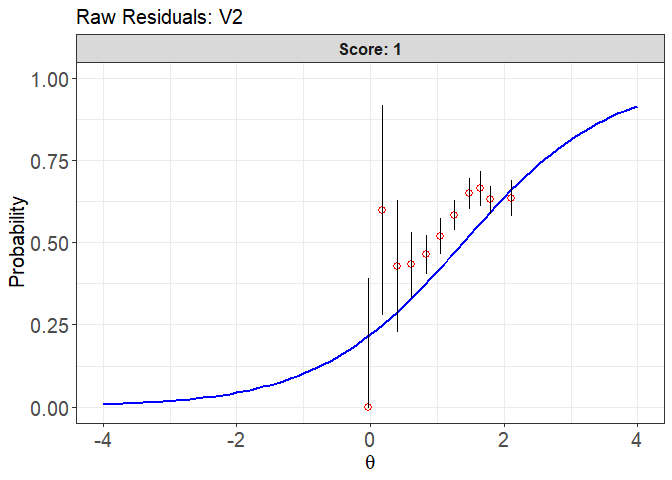
#>                               theta   N freq.0 freq.1 obs.prop.0 obs.prop.1
#> [-0.1218815,0.08512996] -0.02529272   3      3      0  1.0000000  0.0000000
#> (0.08512996,0.2921415]   0.18431014   5      2      3  0.4000000  0.6000000
#> (0.2921415,0.499153]     0.39488272  14      8      6  0.5714286  0.4285714
#> (0.499153,0.7061645]     0.60618911  60     34     26  0.5666667  0.4333333
#> (0.7061645,0.913176]     0.83531169 185     99     86  0.5351351  0.4648649
#> (0.913176,1.120187]      1.04723712 240    115    125  0.4791667  0.5208333
#> (1.120187,1.327199]      1.25232143 349    145    204  0.4154728  0.5845272
#> (1.327199,1.53421]       1.47877397 325    114    211  0.3507692  0.6492308
#> (1.53421,1.741222]       1.63898436 246     82    164  0.3333333  0.6666667
#> (1.741222,1.948233]      1.78810197 377    139    238  0.3687003  0.6312997
#> (1.948233,2.155245]      2.11166019 214     78    136  0.3644860  0.6355140
#>                         exp.prob.0 exp.prob.1 raw_resid.0 raw_resid.1
#> [-0.1218815,0.08512996]  0.7841844  0.2158156  0.21581559 -0.21581559
#> (0.08512996,0.2921415]   0.7499556  0.2500444 -0.34995561  0.34995561
#> (0.2921415,0.499153]     0.7121079  0.2878921 -0.14067932  0.14067932
#> (0.499153,0.7061645]     0.6708959  0.3291041 -0.10422928  0.10422928
#> (0.7061645,0.913176]     0.6230537  0.3769463 -0.08791853  0.08791853
#> (0.913176,1.120187]      0.5765337  0.4234663 -0.09736699  0.09736699
#> (1.120187,1.327199]      0.5301760  0.4698240 -0.11470327  0.11470327
#> (1.327199,1.53421]       0.4784096  0.5215904 -0.12764036  0.12764036
#> (1.53421,1.741222]       0.4419993  0.5580007 -0.10866594  0.10866594
#> (1.741222,1.948233]      0.4086532  0.5913468 -0.03995295  0.03995295
#> (1.948233,2.155245]      0.3394647  0.6605353  0.02502128 -0.02502128
#>                               se.0       se.1 std_resid.0 std_resid.1
#> [-0.1218815,0.08512996] 0.23751437 0.23751437   0.9086423  -0.9086423
#> (0.08512996,0.2921415]  0.19366063 0.19366063  -1.8070560   1.8070560
#> (0.2921415,0.499153]    0.12101070 0.12101070  -1.1625362   1.1625362
#> (0.499153,0.7061645]    0.06066226 0.06066226  -1.7181899   1.7181899
#> (0.7061645,0.913176]    0.03563007 0.03563007  -2.4675377   2.4675377
#> (0.913176,1.120187]     0.03189453 0.03189453  -3.0527806   3.0527806
#> (1.120187,1.327199]     0.02671560 0.02671560  -4.2934941   4.2934941
#> (1.327199,1.53421]      0.02770914 0.02770914  -4.6064351   4.6064351
#> (1.53421,1.741222]      0.03166362 0.03166362  -3.4318859   3.4318859
#> (1.741222,1.948233]     0.02531791 0.02531791  -1.5780508   1.5780508
#> (1.948233,2.155245]     0.03236968 0.03236968   0.7729850  -0.7729850
#>                         raw.resid.0 raw.resid.1     se.0.1     se.1.1
#> [-0.1218815,0.08512996]  0.21581559 -0.21581559 0.23751437 0.23751437
#> (0.08512996,0.2921415]  -0.34995561  0.34995561 0.19366063 0.19366063
#> (0.2921415,0.499153]    -0.14067932  0.14067932 0.12101070 0.12101070
#> (0.499153,0.7061645]    -0.10422928  0.10422928 0.06066226 0.06066226
#> (0.7061645,0.913176]    -0.08791853  0.08791853 0.03563007 0.03563007
#> (0.913176,1.120187]     -0.09736699  0.09736699 0.03189453 0.03189453
#> (1.120187,1.327199]     -0.11470327  0.11470327 0.02671560 0.02671560
#> (1.327199,1.53421]      -0.12764036  0.12764036 0.02770914 0.02770914
#> (1.53421,1.741222]      -0.10866594  0.10866594 0.03166362 0.03166362
#> (1.741222,1.948233]     -0.03995295  0.03995295 0.02531791 0.02531791
#> (1.948233,2.155245]      0.02502128 -0.02502128 0.03236968 0.03236968
#>                         std.resid.0 std.resid.1
#> [-0.1218815,0.08512996]   0.9086423  -0.9086423
#> (0.08512996,0.2921415]   -1.8070560   1.8070560
#> (0.2921415,0.499153]     -1.1625362   1.1625362
#> (0.499153,0.7061645]     -1.7181899   1.7181899
#> (0.7061645,0.913176]     -2.4675377   2.4675377
#> (0.913176,1.120187]      -3.0527806   3.0527806
#> (1.120187,1.327199]      -4.2934941   4.2934941
#> (1.327199,1.53421]       -4.6064351   4.6064351
#> (1.53421,1.741222]       -3.4318859   3.4318859
#> (1.741222,1.948233]      -1.5780508   1.5780508
#> (1.948233,2.155245]       0.7729850  -0.7729850

# (3) the standardized residual plots using the object "fit1"
plot(x=fit1, item.loc=113, type = "sr", ci.method = "wald",  ylim.sr.adjust=TRUE)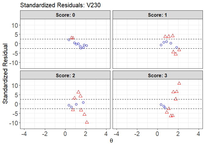
#>                           theta   N freq.0 freq.1 freq.2 freq.3 obs.prop.0
#> [0.3564295,0.5199582] 0.3564295   1      1      0      0      0 1.00000000
#> (0.5199582,0.6834869] 0.6081321   5      3      2      0      0 0.60000000
#> (0.6834869,0.8470155] 0.7400138  15      5     10      0      0 0.33333333
#> (0.8470155,1.010544]  0.8866202  55      5     15     34      1 0.09090909
#> (1.010544,1.174073]   1.0821064 133      6     40     53     34 0.04511278
#> (1.174073,1.337602]   1.2832293 260      8     37    153     62 0.03076923
#> (1.337602,1.50113]    1.4747336  98      0     23     57     18 0.00000000
#> (1.50113,1.664659]    1.5311735 306      0      7     85    214 0.00000000
#> (1.664659,1.828188]   1.7632607 418      0      0    145    273 0.00000000
#> (1.828188,1.991716]   1.8577191  69      0      0      0     69 0.00000000
#> (1.991716,2.155245]   2.1021956 263      0      0      0    263 0.00000000
#>                       obs.prop.1 obs.prop.2 obs.prop.3  exp.prob.0 exp.prob.1
#> [0.3564295,0.5199582] 0.00000000  0.0000000 0.00000000 0.196511833 0.31299790
#> (0.5199582,0.6834869] 0.40000000  0.0000000 0.00000000 0.130431315 0.27025065
#> (0.6834869,0.8470155] 0.66666667  0.0000000 0.00000000 0.102631449 0.24407213
#> (0.8470155,1.010544]  0.27272727  0.6181818 0.01818182 0.077129446 0.21379299
#> (1.010544,1.174073]   0.30075188  0.3984962 0.25563910 0.051169395 0.17398130
#> (1.174073,1.337602]   0.14230769  0.5884615 0.23846154 0.032494074 0.13632441
#> (1.337602,1.50113]    0.23469388  0.5816327 0.18367347 0.020534959 0.10523862
#> (1.50113,1.664659]    0.02287582  0.2777778 0.69934641 0.017857642 0.09707782
#> (1.664659,1.828188]   0.00000000  0.3468900 0.65311005 0.009866868 0.06836048
#> (1.828188,1.991716]   0.00000000  0.0000000 1.00000000 0.007690015 0.05880602
#> (1.991716,2.155245]   0.00000000  0.0000000 1.00000000 0.003962699 0.03912356
#>                       exp.prob.2 exp.prob.3  raw_resid.0  raw_resid.1
#> [0.3564295,0.5199582]  0.3472692  0.1432210  0.803488167 -0.312997903
#> (0.5199582,0.6834869]  0.3900531  0.2092649  0.469568685  0.129749354
#> (0.6834869,0.8470155]  0.4043226  0.2489738  0.230701885  0.422594537
#> (0.8470155,1.010544]   0.4127992  0.2962784  0.013779645  0.058934282
#> (1.010544,1.174073]    0.4120662  0.3627831 -0.006056613  0.126770584
#> (1.174073,1.337602]    0.3983962  0.4327853 -0.001724843  0.005983284
#> (1.337602,1.50113]     0.3756891  0.4985373 -0.020534959  0.129455259
#> (1.50113,1.664659]     0.3676106  0.5174539 -0.017857642 -0.074201998
#> (1.664659,1.828188]    0.3299158  0.5918569 -0.009866868 -0.068360484
#> (1.828188,1.991716]    0.3132481  0.6202558 -0.007690015 -0.058806016
#> (1.991716,2.155245]    0.2690653  0.6878484 -0.003962699 -0.039123555
#>                       raw_resid.2 raw_resid.3        se.0       se.1       se.2
#> [0.3564295,0.5199582] -0.34726922 -0.14322104 0.397359953 0.46371351 0.47610220
#> (0.5199582,0.6834869] -0.39005312 -0.20926492 0.150611412 0.19860274 0.21813376
#> (0.6834869,0.8470155] -0.40432265 -0.24897378 0.078357401 0.11090564 0.12671381
#> (0.8470155,1.010544]   0.20538261 -0.27809653 0.035974863 0.05528201 0.06638675
#> (1.010544,1.174073]   -0.01356995 -0.10714402 0.019106171 0.03287157 0.04267975
#> (1.174073,1.337602]    0.19006531 -0.19432375 0.010996190 0.02128019 0.03036171
#> (1.337602,1.50113]     0.20594357 -0.31486387 0.014326112 0.03099761 0.04892172
#> (1.50113,1.664659]    -0.08983281  0.18189246 0.007570744 0.01692484 0.02756294
#> (1.664659,1.828188]    0.01697418  0.06125317 0.004834464 0.01234350 0.02299737
#> (1.828188,1.991716]   -0.31324812  0.37974416 0.010516294 0.02832213 0.05583668
#> (1.991716,2.155245]   -0.26906531  0.31215156 0.003873963 0.01195570 0.02734578
#>                             se.3 std_resid.0 std_resid.1 std_resid.2
#> [0.3564295,0.5199582] 0.35029812   2.0220663  -0.6749812  -0.7294006
#> (0.5199582,0.6834869] 0.18191928   3.1177497   0.6533110  -1.7881373
#> (0.6834869,0.8470155] 0.11165000   2.9442258   3.8103971  -3.1908333
#> (0.8470155,1.010544]  0.06156999   0.3830354   1.0660662   3.0937290
#> (1.010544,1.174073]   0.04169091  -0.3169978   3.8565422  -0.3179482
#> (1.174073,1.337602]   0.03072722  -0.1568583   0.2811669   6.2600333
#> (1.337602,1.50113]    0.05050741  -1.4333937   4.1762987   4.2096551
#> (1.50113,1.664659]    0.02856568  -2.3587698  -4.3842081  -3.2591881
#> (1.664659,1.828188]   0.02403956  -2.0409436  -5.5381760   0.7380923
#> (1.828188,1.991716]   0.05842604  -0.7312476  -2.0763275  -5.6100775
#> (1.991716,2.155245]   0.02857270  -1.0229057  -3.2723764  -9.8393733
#>                       std_resid.3  raw.resid.0  raw.resid.1 raw.resid.2
#> [0.3564295,0.5199582]  -0.4088547  0.803488167 -0.312997903 -0.34726922
#> (0.5199582,0.6834869]  -1.1503175  0.469568685  0.129749354 -0.39005312
#> (0.6834869,0.8470155]  -2.2299488  0.230701885  0.422594537 -0.40432265
#> (0.8470155,1.010544]   -4.5167547  0.013779645  0.058934282  0.20538261
#> (1.010544,1.174073]    -2.5699613 -0.006056613  0.126770584 -0.01356995
#> (1.174073,1.337602]    -6.3241558 -0.001724843  0.005983284  0.19006531
#> (1.337602,1.50113]     -6.2340132 -0.020534959  0.129455259  0.20594357
#> (1.50113,1.664659]      6.3675177 -0.017857642 -0.074201998 -0.08983281
#> (1.664659,1.828188]     2.5480159 -0.009866868 -0.068360484  0.01697418
#> (1.828188,1.991716]     6.4995706 -0.007690015 -0.058806016 -0.31324812
#> (1.991716,2.155245]    10.9248190 -0.003962699 -0.039123555 -0.26906531
#>                       raw.resid.3      se.0.1     se.1.1     se.2.1     se.3.1
#> [0.3564295,0.5199582] -0.14322104 0.397359953 0.46371351 0.47610220 0.35029812
#> (0.5199582,0.6834869] -0.20926492 0.150611412 0.19860274 0.21813376 0.18191928
#> (0.6834869,0.8470155] -0.24897378 0.078357401 0.11090564 0.12671381 0.11165000
#> (0.8470155,1.010544]  -0.27809653 0.035974863 0.05528201 0.06638675 0.06156999
#> (1.010544,1.174073]   -0.10714402 0.019106171 0.03287157 0.04267975 0.04169091
#> (1.174073,1.337602]   -0.19432375 0.010996190 0.02128019 0.03036171 0.03072722
#> (1.337602,1.50113]    -0.31486387 0.014326112 0.03099761 0.04892172 0.05050741
#> (1.50113,1.664659]     0.18189246 0.007570744 0.01692484 0.02756294 0.02856568
#> (1.664659,1.828188]    0.06125317 0.004834464 0.01234350 0.02299737 0.02403956
#> (1.828188,1.991716]    0.37974416 0.010516294 0.02832213 0.05583668 0.05842604
#> (1.991716,2.155245]    0.31215156 0.003873963 0.01195570 0.02734578 0.02857270
#>                       std.resid.0 std.resid.1 std.resid.2 std.resid.3
#> [0.3564295,0.5199582]   2.0220663  -0.6749812  -0.7294006  -0.4088547
#> (0.5199582,0.6834869]   3.1177497   0.6533110  -1.7881373  -1.1503175
#> (0.6834869,0.8470155]   2.9442258   3.8103971  -3.1908333  -2.2299488
#> (0.8470155,1.010544]    0.3830354   1.0660662   3.0937290  -4.5167547
#> (1.010544,1.174073]    -0.3169978   3.8565422  -0.3179482  -2.5699613
#> (1.174073,1.337602]    -0.1568583   0.2811669   6.2600333  -6.3241558
#> (1.337602,1.50113]     -1.4333937   4.1762987   4.2096551  -6.2340132
#> (1.50113,1.664659]     -2.3587698  -4.3842081  -3.2591881   6.3675177
#> (1.664659,1.828188]    -2.0409436  -5.5381760   0.7380923   2.5480159
#> (1.828188,1.991716]    -0.7312476  -2.0763275  -5.6100775   6.4995706
#> (1.991716,2.155245]    -1.0229057  -3.2723764  -9.8393733  10.9248190

# 2. the polytomous item
# (1) both raw and standardized residual plots using the object "fit1"
plot(x=fit1, item.loc=113, type = "both", ci.method = "wald",  ylim.sr.adjust=TRUE)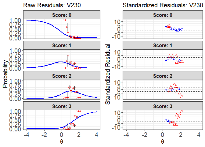
#>                           theta   N freq.0 freq.1 freq.2 freq.3 obs.prop.0
#> [0.3564295,0.5199582] 0.3564295   1      1      0      0      0 1.00000000
#> (0.5199582,0.6834869] 0.6081321   5      3      2      0      0 0.60000000
#> (0.6834869,0.8470155] 0.7400138  15      5     10      0      0 0.33333333
#> (0.8470155,1.010544]  0.8866202  55      5     15     34      1 0.09090909
#> (1.010544,1.174073]   1.0821064 133      6     40     53     34 0.04511278
#> (1.174073,1.337602]   1.2832293 260      8     37    153     62 0.03076923
#> (1.337602,1.50113]    1.4747336  98      0     23     57     18 0.00000000
#> (1.50113,1.664659]    1.5311735 306      0      7     85    214 0.00000000
#> (1.664659,1.828188]   1.7632607 418      0      0    145    273 0.00000000
#> (1.828188,1.991716]   1.8577191  69      0      0      0     69 0.00000000
#> (1.991716,2.155245]   2.1021956 263      0      0      0    263 0.00000000
#>                       obs.prop.1 obs.prop.2 obs.prop.3  exp.prob.0 exp.prob.1
#> [0.3564295,0.5199582] 0.00000000  0.0000000 0.00000000 0.196511833 0.31299790
#> (0.5199582,0.6834869] 0.40000000  0.0000000 0.00000000 0.130431315 0.27025065
#> (0.6834869,0.8470155] 0.66666667  0.0000000 0.00000000 0.102631449 0.24407213
#> (0.8470155,1.010544]  0.27272727  0.6181818 0.01818182 0.077129446 0.21379299
#> (1.010544,1.174073]   0.30075188  0.3984962 0.25563910 0.051169395 0.17398130
#> (1.174073,1.337602]   0.14230769  0.5884615 0.23846154 0.032494074 0.13632441
#> (1.337602,1.50113]    0.23469388  0.5816327 0.18367347 0.020534959 0.10523862
#> (1.50113,1.664659]    0.02287582  0.2777778 0.69934641 0.017857642 0.09707782
#> (1.664659,1.828188]   0.00000000  0.3468900 0.65311005 0.009866868 0.06836048
#> (1.828188,1.991716]   0.00000000  0.0000000 1.00000000 0.007690015 0.05880602
#> (1.991716,2.155245]   0.00000000  0.0000000 1.00000000 0.003962699 0.03912356
#>                       exp.prob.2 exp.prob.3  raw_resid.0  raw_resid.1
#> [0.3564295,0.5199582]  0.3472692  0.1432210  0.803488167 -0.312997903
#> (0.5199582,0.6834869]  0.3900531  0.2092649  0.469568685  0.129749354
#> (0.6834869,0.8470155]  0.4043226  0.2489738  0.230701885  0.422594537
#> (0.8470155,1.010544]   0.4127992  0.2962784  0.013779645  0.058934282
#> (1.010544,1.174073]    0.4120662  0.3627831 -0.006056613  0.126770584
#> (1.174073,1.337602]    0.3983962  0.4327853 -0.001724843  0.005983284
#> (1.337602,1.50113]     0.3756891  0.4985373 -0.020534959  0.129455259
#> (1.50113,1.664659]     0.3676106  0.5174539 -0.017857642 -0.074201998
#> (1.664659,1.828188]    0.3299158  0.5918569 -0.009866868 -0.068360484
#> (1.828188,1.991716]    0.3132481  0.6202558 -0.007690015 -0.058806016
#> (1.991716,2.155245]    0.2690653  0.6878484 -0.003962699 -0.039123555
#>                       raw_resid.2 raw_resid.3        se.0       se.1       se.2
#> [0.3564295,0.5199582] -0.34726922 -0.14322104 0.397359953 0.46371351 0.47610220
#> (0.5199582,0.6834869] -0.39005312 -0.20926492 0.150611412 0.19860274 0.21813376
#> (0.6834869,0.8470155] -0.40432265 -0.24897378 0.078357401 0.11090564 0.12671381
#> (0.8470155,1.010544]   0.20538261 -0.27809653 0.035974863 0.05528201 0.06638675
#> (1.010544,1.174073]   -0.01356995 -0.10714402 0.019106171 0.03287157 0.04267975
#> (1.174073,1.337602]    0.19006531 -0.19432375 0.010996190 0.02128019 0.03036171
#> (1.337602,1.50113]     0.20594357 -0.31486387 0.014326112 0.03099761 0.04892172
#> (1.50113,1.664659]    -0.08983281  0.18189246 0.007570744 0.01692484 0.02756294
#> (1.664659,1.828188]    0.01697418  0.06125317 0.004834464 0.01234350 0.02299737
#> (1.828188,1.991716]   -0.31324812  0.37974416 0.010516294 0.02832213 0.05583668
#> (1.991716,2.155245]   -0.26906531  0.31215156 0.003873963 0.01195570 0.02734578
#>                             se.3 std_resid.0 std_resid.1 std_resid.2
#> [0.3564295,0.5199582] 0.35029812   2.0220663  -0.6749812  -0.7294006
#> (0.5199582,0.6834869] 0.18191928   3.1177497   0.6533110  -1.7881373
#> (0.6834869,0.8470155] 0.11165000   2.9442258   3.8103971  -3.1908333
#> (0.8470155,1.010544]  0.06156999   0.3830354   1.0660662   3.0937290
#> (1.010544,1.174073]   0.04169091  -0.3169978   3.8565422  -0.3179482
#> (1.174073,1.337602]   0.03072722  -0.1568583   0.2811669   6.2600333
#> (1.337602,1.50113]    0.05050741  -1.4333937   4.1762987   4.2096551
#> (1.50113,1.664659]    0.02856568  -2.3587698  -4.3842081  -3.2591881
#> (1.664659,1.828188]   0.02403956  -2.0409436  -5.5381760   0.7380923
#> (1.828188,1.991716]   0.05842604  -0.7312476  -2.0763275  -5.6100775
#> (1.991716,2.155245]   0.02857270  -1.0229057  -3.2723764  -9.8393733
#>                       std_resid.3  raw.resid.0  raw.resid.1 raw.resid.2
#> [0.3564295,0.5199582]  -0.4088547  0.803488167 -0.312997903 -0.34726922
#> (0.5199582,0.6834869]  -1.1503175  0.469568685  0.129749354 -0.39005312
#> (0.6834869,0.8470155]  -2.2299488  0.230701885  0.422594537 -0.40432265
#> (0.8470155,1.010544]   -4.5167547  0.013779645  0.058934282  0.20538261
#> (1.010544,1.174073]    -2.5699613 -0.006056613  0.126770584 -0.01356995
#> (1.174073,1.337602]    -6.3241558 -0.001724843  0.005983284  0.19006531
#> (1.337602,1.50113]     -6.2340132 -0.020534959  0.129455259  0.20594357
#> (1.50113,1.664659]      6.3675177 -0.017857642 -0.074201998 -0.08983281
#> (1.664659,1.828188]     2.5480159 -0.009866868 -0.068360484  0.01697418
#> (1.828188,1.991716]     6.4995706 -0.007690015 -0.058806016 -0.31324812
#> (1.991716,2.155245]    10.9248190 -0.003962699 -0.039123555 -0.26906531
#>                       raw.resid.3      se.0.1     se.1.1     se.2.1     se.3.1
#> [0.3564295,0.5199582] -0.14322104 0.397359953 0.46371351 0.47610220 0.35029812
#> (0.5199582,0.6834869] -0.20926492 0.150611412 0.19860274 0.21813376 0.18191928
#> (0.6834869,0.8470155] -0.24897378 0.078357401 0.11090564 0.12671381 0.11165000
#> (0.8470155,1.010544]  -0.27809653 0.035974863 0.05528201 0.06638675 0.06156999
#> (1.010544,1.174073]   -0.10714402 0.019106171 0.03287157 0.04267975 0.04169091
#> (1.174073,1.337602]   -0.19432375 0.010996190 0.02128019 0.03036171 0.03072722
#> (1.337602,1.50113]    -0.31486387 0.014326112 0.03099761 0.04892172 0.05050741
#> (1.50113,1.664659]     0.18189246 0.007570744 0.01692484 0.02756294 0.02856568
#> (1.664659,1.828188]    0.06125317 0.004834464 0.01234350 0.02299737 0.02403956
#> (1.828188,1.991716]    0.37974416 0.010516294 0.02832213 0.05583668 0.05842604
#> (1.991716,2.155245]    0.31215156 0.003873963 0.01195570 0.02734578 0.02857270
#>                       std.resid.0 std.resid.1 std.resid.2 std.resid.3
#> [0.3564295,0.5199582]   2.0220663  -0.6749812  -0.7294006  -0.4088547
#> (0.5199582,0.6834869]   3.1177497   0.6533110  -1.7881373  -1.1503175
#> (0.6834869,0.8470155]   2.9442258   3.8103971  -3.1908333  -2.2299488
#> (0.8470155,1.010544]    0.3830354   1.0660662   3.0937290  -4.5167547
#> (1.010544,1.174073]    -0.3169978   3.8565422  -0.3179482  -2.5699613
#> (1.174073,1.337602]    -0.1568583   0.2811669   6.2600333  -6.3241558
#> (1.337602,1.50113]     -1.4333937   4.1762987   4.2096551  -6.2340132
#> (1.50113,1.664659]     -2.3587698  -4.3842081  -3.2591881   6.3675177
#> (1.664659,1.828188]    -2.0409436  -5.5381760   0.7380923   2.5480159
#> (1.828188,1.991716]    -0.7312476  -2.0763275  -5.6100775   6.4995706
#> (1.991716,2.155245]    -1.0229057  -3.2723764  -9.8393733  10.9248190

# (2) the raw residual plots using the object "fit1"
plot(x=fit1, item.loc=113, type = "icc", ci.method = "wald", layout.col=2, ylim.sr.adjust=TRUE)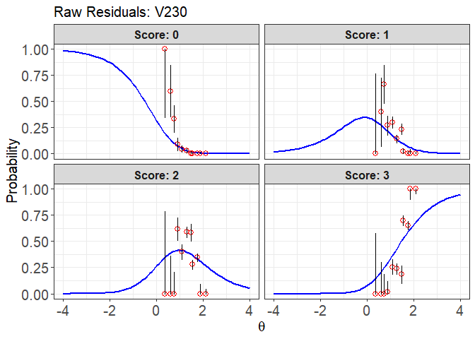
#>                           theta   N freq.0 freq.1 freq.2 freq.3 obs.prop.0
#> [0.3564295,0.5199582] 0.3564295   1      1      0      0      0 1.00000000
#> (0.5199582,0.6834869] 0.6081321   5      3      2      0      0 0.60000000
#> (0.6834869,0.8470155] 0.7400138  15      5     10      0      0 0.33333333
#> (0.8470155,1.010544]  0.8866202  55      5     15     34      1 0.09090909
#> (1.010544,1.174073]   1.0821064 133      6     40     53     34 0.04511278
#> (1.174073,1.337602]   1.2832293 260      8     37    153     62 0.03076923
#> (1.337602,1.50113]    1.4747336  98      0     23     57     18 0.00000000
#> (1.50113,1.664659]    1.5311735 306      0      7     85    214 0.00000000
#> (1.664659,1.828188]   1.7632607 418      0      0    145    273 0.00000000
#> (1.828188,1.991716]   1.8577191  69      0      0      0     69 0.00000000
#> (1.991716,2.155245]   2.1021956 263      0      0      0    263 0.00000000
#>                       obs.prop.1 obs.prop.2 obs.prop.3  exp.prob.0 exp.prob.1
#> [0.3564295,0.5199582] 0.00000000  0.0000000 0.00000000 0.196511833 0.31299790
#> (0.5199582,0.6834869] 0.40000000  0.0000000 0.00000000 0.130431315 0.27025065
#> (0.6834869,0.8470155] 0.66666667  0.0000000 0.00000000 0.102631449 0.24407213
#> (0.8470155,1.010544]  0.27272727  0.6181818 0.01818182 0.077129446 0.21379299
#> (1.010544,1.174073]   0.30075188  0.3984962 0.25563910 0.051169395 0.17398130
#> (1.174073,1.337602]   0.14230769  0.5884615 0.23846154 0.032494074 0.13632441
#> (1.337602,1.50113]    0.23469388  0.5816327 0.18367347 0.020534959 0.10523862
#> (1.50113,1.664659]    0.02287582  0.2777778 0.69934641 0.017857642 0.09707782
#> (1.664659,1.828188]   0.00000000  0.3468900 0.65311005 0.009866868 0.06836048
#> (1.828188,1.991716]   0.00000000  0.0000000 1.00000000 0.007690015 0.05880602
#> (1.991716,2.155245]   0.00000000  0.0000000 1.00000000 0.003962699 0.03912356
#>                       exp.prob.2 exp.prob.3  raw_resid.0  raw_resid.1
#> [0.3564295,0.5199582]  0.3472692  0.1432210  0.803488167 -0.312997903
#> (0.5199582,0.6834869]  0.3900531  0.2092649  0.469568685  0.129749354
#> (0.6834869,0.8470155]  0.4043226  0.2489738  0.230701885  0.422594537
#> (0.8470155,1.010544]   0.4127992  0.2962784  0.013779645  0.058934282
#> (1.010544,1.174073]    0.4120662  0.3627831 -0.006056613  0.126770584
#> (1.174073,1.337602]    0.3983962  0.4327853 -0.001724843  0.005983284
#> (1.337602,1.50113]     0.3756891  0.4985373 -0.020534959  0.129455259
#> (1.50113,1.664659]     0.3676106  0.5174539 -0.017857642 -0.074201998
#> (1.664659,1.828188]    0.3299158  0.5918569 -0.009866868 -0.068360484
#> (1.828188,1.991716]    0.3132481  0.6202558 -0.007690015 -0.058806016
#> (1.991716,2.155245]    0.2690653  0.6878484 -0.003962699 -0.039123555
#>                       raw_resid.2 raw_resid.3        se.0       se.1       se.2
#> [0.3564295,0.5199582] -0.34726922 -0.14322104 0.397359953 0.46371351 0.47610220
#> (0.5199582,0.6834869] -0.39005312 -0.20926492 0.150611412 0.19860274 0.21813376
#> (0.6834869,0.8470155] -0.40432265 -0.24897378 0.078357401 0.11090564 0.12671381
#> (0.8470155,1.010544]   0.20538261 -0.27809653 0.035974863 0.05528201 0.06638675
#> (1.010544,1.174073]   -0.01356995 -0.10714402 0.019106171 0.03287157 0.04267975
#> (1.174073,1.337602]    0.19006531 -0.19432375 0.010996190 0.02128019 0.03036171
#> (1.337602,1.50113]     0.20594357 -0.31486387 0.014326112 0.03099761 0.04892172
#> (1.50113,1.664659]    -0.08983281  0.18189246 0.007570744 0.01692484 0.02756294
#> (1.664659,1.828188]    0.01697418  0.06125317 0.004834464 0.01234350 0.02299737
#> (1.828188,1.991716]   -0.31324812  0.37974416 0.010516294 0.02832213 0.05583668
#> (1.991716,2.155245]   -0.26906531  0.31215156 0.003873963 0.01195570 0.02734578
#>                             se.3 std_resid.0 std_resid.1 std_resid.2
#> [0.3564295,0.5199582] 0.35029812   2.0220663  -0.6749812  -0.7294006
#> (0.5199582,0.6834869] 0.18191928   3.1177497   0.6533110  -1.7881373
#> (0.6834869,0.8470155] 0.11165000   2.9442258   3.8103971  -3.1908333
#> (0.8470155,1.010544]  0.06156999   0.3830354   1.0660662   3.0937290
#> (1.010544,1.174073]   0.04169091  -0.3169978   3.8565422  -0.3179482
#> (1.174073,1.337602]   0.03072722  -0.1568583   0.2811669   6.2600333
#> (1.337602,1.50113]    0.05050741  -1.4333937   4.1762987   4.2096551
#> (1.50113,1.664659]    0.02856568  -2.3587698  -4.3842081  -3.2591881
#> (1.664659,1.828188]   0.02403956  -2.0409436  -5.5381760   0.7380923
#> (1.828188,1.991716]   0.05842604  -0.7312476  -2.0763275  -5.6100775
#> (1.991716,2.155245]   0.02857270  -1.0229057  -3.2723764  -9.8393733
#>                       std_resid.3  raw.resid.0  raw.resid.1 raw.resid.2
#> [0.3564295,0.5199582]  -0.4088547  0.803488167 -0.312997903 -0.34726922
#> (0.5199582,0.6834869]  -1.1503175  0.469568685  0.129749354 -0.39005312
#> (0.6834869,0.8470155]  -2.2299488  0.230701885  0.422594537 -0.40432265
#> (0.8470155,1.010544]   -4.5167547  0.013779645  0.058934282  0.20538261
#> (1.010544,1.174073]    -2.5699613 -0.006056613  0.126770584 -0.01356995
#> (1.174073,1.337602]    -6.3241558 -0.001724843  0.005983284  0.19006531
#> (1.337602,1.50113]     -6.2340132 -0.020534959  0.129455259  0.20594357
#> (1.50113,1.664659]      6.3675177 -0.017857642 -0.074201998 -0.08983281
#> (1.664659,1.828188]     2.5480159 -0.009866868 -0.068360484  0.01697418
#> (1.828188,1.991716]     6.4995706 -0.007690015 -0.058806016 -0.31324812
#> (1.991716,2.155245]    10.9248190 -0.003962699 -0.039123555 -0.26906531
#>                       raw.resid.3      se.0.1     se.1.1     se.2.1     se.3.1
#> [0.3564295,0.5199582] -0.14322104 0.397359953 0.46371351 0.47610220 0.35029812
#> (0.5199582,0.6834869] -0.20926492 0.150611412 0.19860274 0.21813376 0.18191928
#> (0.6834869,0.8470155] -0.24897378 0.078357401 0.11090564 0.12671381 0.11165000
#> (0.8470155,1.010544]  -0.27809653 0.035974863 0.05528201 0.06638675 0.06156999
#> (1.010544,1.174073]   -0.10714402 0.019106171 0.03287157 0.04267975 0.04169091
#> (1.174073,1.337602]   -0.19432375 0.010996190 0.02128019 0.03036171 0.03072722
#> (1.337602,1.50113]    -0.31486387 0.014326112 0.03099761 0.04892172 0.05050741
#> (1.50113,1.664659]     0.18189246 0.007570744 0.01692484 0.02756294 0.02856568
#> (1.664659,1.828188]    0.06125317 0.004834464 0.01234350 0.02299737 0.02403956
#> (1.828188,1.991716]    0.37974416 0.010516294 0.02832213 0.05583668 0.05842604
#> (1.991716,2.155245]    0.31215156 0.003873963 0.01195570 0.02734578 0.02857270
#>                       std.resid.0 std.resid.1 std.resid.2 std.resid.3
#> [0.3564295,0.5199582]   2.0220663  -0.6749812  -0.7294006  -0.4088547
#> (0.5199582,0.6834869]   3.1177497   0.6533110  -1.7881373  -1.1503175
#> (0.6834869,0.8470155]   2.9442258   3.8103971  -3.1908333  -2.2299488
#> (0.8470155,1.010544]    0.3830354   1.0660662   3.0937290  -4.5167547
#> (1.010544,1.174073]    -0.3169978   3.8565422  -0.3179482  -2.5699613
#> (1.174073,1.337602]    -0.1568583   0.2811669   6.2600333  -6.3241558
#> (1.337602,1.50113]     -1.4333937   4.1762987   4.2096551  -6.2340132
#> (1.50113,1.664659]     -2.3587698  -4.3842081  -3.2591881   6.3675177
#> (1.664659,1.828188]    -2.0409436  -5.5381760   0.7380923   2.5480159
#> (1.828188,1.991716]    -0.7312476  -2.0763275  -5.6100775   6.4995706
#> (1.991716,2.155245]    -1.0229057  -3.2723764  -9.8393733  10.9248190

# (3) the standardized residual plots using the object "fit1"
plot(x=fit1, item.loc=113, type = "sr", ci.method = "wald", layout.col=4, ylim.sr.adjust=TRUE)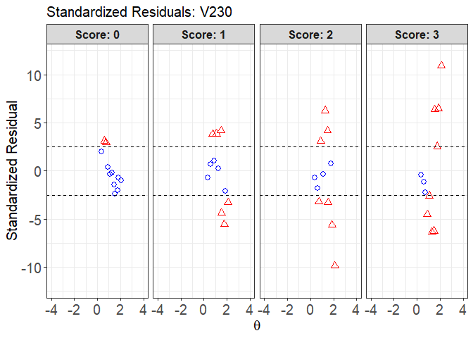
#>                           theta   N freq.0 freq.1 freq.2 freq.3 obs.prop.0
#> [0.3564295,0.5199582] 0.3564295   1      1      0      0      0 1.00000000
#> (0.5199582,0.6834869] 0.6081321   5      3      2      0      0 0.60000000
#> (0.6834869,0.8470155] 0.7400138  15      5     10      0      0 0.33333333
#> (0.8470155,1.010544]  0.8866202  55      5     15     34      1 0.09090909
#> (1.010544,1.174073]   1.0821064 133      6     40     53     34 0.04511278
#> (1.174073,1.337602]   1.2832293 260      8     37    153     62 0.03076923
#> (1.337602,1.50113]    1.4747336  98      0     23     57     18 0.00000000
#> (1.50113,1.664659]    1.5311735 306      0      7     85    214 0.00000000
#> (1.664659,1.828188]   1.7632607 418      0      0    145    273 0.00000000
#> (1.828188,1.991716]   1.8577191  69      0      0      0     69 0.00000000
#> (1.991716,2.155245]   2.1021956 263      0      0      0    263 0.00000000
#>                       obs.prop.1 obs.prop.2 obs.prop.3  exp.prob.0 exp.prob.1
#> [0.3564295,0.5199582] 0.00000000  0.0000000 0.00000000 0.196511833 0.31299790
#> (0.5199582,0.6834869] 0.40000000  0.0000000 0.00000000 0.130431315 0.27025065
#> (0.6834869,0.8470155] 0.66666667  0.0000000 0.00000000 0.102631449 0.24407213
#> (0.8470155,1.010544]  0.27272727  0.6181818 0.01818182 0.077129446 0.21379299
#> (1.010544,1.174073]   0.30075188  0.3984962 0.25563910 0.051169395 0.17398130
#> (1.174073,1.337602]   0.14230769  0.5884615 0.23846154 0.032494074 0.13632441
#> (1.337602,1.50113]    0.23469388  0.5816327 0.18367347 0.020534959 0.10523862
#> (1.50113,1.664659]    0.02287582  0.2777778 0.69934641 0.017857642 0.09707782
#> (1.664659,1.828188]   0.00000000  0.3468900 0.65311005 0.009866868 0.06836048
#> (1.828188,1.991716]   0.00000000  0.0000000 1.00000000 0.007690015 0.05880602
#> (1.991716,2.155245]   0.00000000  0.0000000 1.00000000 0.003962699 0.03912356
#>                       exp.prob.2 exp.prob.3  raw_resid.0  raw_resid.1
#> [0.3564295,0.5199582]  0.3472692  0.1432210  0.803488167 -0.312997903
#> (0.5199582,0.6834869]  0.3900531  0.2092649  0.469568685  0.129749354
#> (0.6834869,0.8470155]  0.4043226  0.2489738  0.230701885  0.422594537
#> (0.8470155,1.010544]   0.4127992  0.2962784  0.013779645  0.058934282
#> (1.010544,1.174073]    0.4120662  0.3627831 -0.006056613  0.126770584
#> (1.174073,1.337602]    0.3983962  0.4327853 -0.001724843  0.005983284
#> (1.337602,1.50113]     0.3756891  0.4985373 -0.020534959  0.129455259
#> (1.50113,1.664659]     0.3676106  0.5174539 -0.017857642 -0.074201998
#> (1.664659,1.828188]    0.3299158  0.5918569 -0.009866868 -0.068360484
#> (1.828188,1.991716]    0.3132481  0.6202558 -0.007690015 -0.058806016
#> (1.991716,2.155245]    0.2690653  0.6878484 -0.003962699 -0.039123555
#>                       raw_resid.2 raw_resid.3        se.0       se.1       se.2
#> [0.3564295,0.5199582] -0.34726922 -0.14322104 0.397359953 0.46371351 0.47610220
#> (0.5199582,0.6834869] -0.39005312 -0.20926492 0.150611412 0.19860274 0.21813376
#> (0.6834869,0.8470155] -0.40432265 -0.24897378 0.078357401 0.11090564 0.12671381
#> (0.8470155,1.010544]   0.20538261 -0.27809653 0.035974863 0.05528201 0.06638675
#> (1.010544,1.174073]   -0.01356995 -0.10714402 0.019106171 0.03287157 0.04267975
#> (1.174073,1.337602]    0.19006531 -0.19432375 0.010996190 0.02128019 0.03036171
#> (1.337602,1.50113]     0.20594357 -0.31486387 0.014326112 0.03099761 0.04892172
#> (1.50113,1.664659]    -0.08983281  0.18189246 0.007570744 0.01692484 0.02756294
#> (1.664659,1.828188]    0.01697418  0.06125317 0.004834464 0.01234350 0.02299737
#> (1.828188,1.991716]   -0.31324812  0.37974416 0.010516294 0.02832213 0.05583668
#> (1.991716,2.155245]   -0.26906531  0.31215156 0.003873963 0.01195570 0.02734578
#>                             se.3 std_resid.0 std_resid.1 std_resid.2
#> [0.3564295,0.5199582] 0.35029812   2.0220663  -0.6749812  -0.7294006
#> (0.5199582,0.6834869] 0.18191928   3.1177497   0.6533110  -1.7881373
#> (0.6834869,0.8470155] 0.11165000   2.9442258   3.8103971  -3.1908333
#> (0.8470155,1.010544]  0.06156999   0.3830354   1.0660662   3.0937290
#> (1.010544,1.174073]   0.04169091  -0.3169978   3.8565422  -0.3179482
#> (1.174073,1.337602]   0.03072722  -0.1568583   0.2811669   6.2600333
#> (1.337602,1.50113]    0.05050741  -1.4333937   4.1762987   4.2096551
#> (1.50113,1.664659]    0.02856568  -2.3587698  -4.3842081  -3.2591881
#> (1.664659,1.828188]   0.02403956  -2.0409436  -5.5381760   0.7380923
#> (1.828188,1.991716]   0.05842604  -0.7312476  -2.0763275  -5.6100775
#> (1.991716,2.155245]   0.02857270  -1.0229057  -3.2723764  -9.8393733
#>                       std_resid.3  raw.resid.0  raw.resid.1 raw.resid.2
#> [0.3564295,0.5199582]  -0.4088547  0.803488167 -0.312997903 -0.34726922
#> (0.5199582,0.6834869]  -1.1503175  0.469568685  0.129749354 -0.39005312
#> (0.6834869,0.8470155]  -2.2299488  0.230701885  0.422594537 -0.40432265
#> (0.8470155,1.010544]   -4.5167547  0.013779645  0.058934282  0.20538261
#> (1.010544,1.174073]    -2.5699613 -0.006056613  0.126770584 -0.01356995
#> (1.174073,1.337602]    -6.3241558 -0.001724843  0.005983284  0.19006531
#> (1.337602,1.50113]     -6.2340132 -0.020534959  0.129455259  0.20594357
#> (1.50113,1.664659]      6.3675177 -0.017857642 -0.074201998 -0.08983281
#> (1.664659,1.828188]     2.5480159 -0.009866868 -0.068360484  0.01697418
#> (1.828188,1.991716]     6.4995706 -0.007690015 -0.058806016 -0.31324812
#> (1.991716,2.155245]    10.9248190 -0.003962699 -0.039123555 -0.26906531
#>                       raw.resid.3      se.0.1     se.1.1     se.2.1     se.3.1
#> [0.3564295,0.5199582] -0.14322104 0.397359953 0.46371351 0.47610220 0.35029812
#> (0.5199582,0.6834869] -0.20926492 0.150611412 0.19860274 0.21813376 0.18191928
#> (0.6834869,0.8470155] -0.24897378 0.078357401 0.11090564 0.12671381 0.11165000
#> (0.8470155,1.010544]  -0.27809653 0.035974863 0.05528201 0.06638675 0.06156999
#> (1.010544,1.174073]   -0.10714402 0.019106171 0.03287157 0.04267975 0.04169091
#> (1.174073,1.337602]   -0.19432375 0.010996190 0.02128019 0.03036171 0.03072722
#> (1.337602,1.50113]    -0.31486387 0.014326112 0.03099761 0.04892172 0.05050741
#> (1.50113,1.664659]     0.18189246 0.007570744 0.01692484 0.02756294 0.02856568
#> (1.664659,1.828188]    0.06125317 0.004834464 0.01234350 0.02299737 0.02403956
#> (1.828188,1.991716]    0.37974416 0.010516294 0.02832213 0.05583668 0.05842604
#> (1.991716,2.155245]    0.31215156 0.003873963 0.01195570 0.02734578 0.02857270
#>                       std.resid.0 std.resid.1 std.resid.2 std.resid.3
#> [0.3564295,0.5199582]   2.0220663  -0.6749812  -0.7294006  -0.4088547
#> (0.5199582,0.6834869]   3.1177497   0.6533110  -1.7881373  -1.1503175
#> (0.6834869,0.8470155]   2.9442258   3.8103971  -3.1908333  -2.2299488
#> (0.8470155,1.010544]    0.3830354   1.0660662   3.0937290  -4.5167547
#> (1.010544,1.174073]    -0.3169978   3.8565422  -0.3179482  -2.5699613
#> (1.174073,1.337602]    -0.1568583   0.2811669   6.2600333  -6.3241558
#> (1.337602,1.50113]     -1.4333937   4.1762987   4.2096551  -6.2340132
#> (1.50113,1.664659]     -2.3587698  -4.3842081  -3.2591881   6.3675177
#> (1.664659,1.828188]    -2.0409436  -5.5381760   0.7380923   2.5480159
#> (1.828188,1.991716]    -0.7312476  -2.0763275  -5.6100775   6.4995706
#> (1.991716,2.155245]    -1.0229057  -3.2723764  -9.8393733  10.9248190