
The R package ‘iglu’ provides functions for outputting relevant metrics for data collected from Continuous Glucose Monitors (CGM). For reference, see “Interpretation of continuous glucose monitoring data: glycemic variability and quality of glycemic control.” Rodbard (2009).
iglu comes with two example datasets: example_data_1_subject and example_data_5_subject. These data are collected using Dexcom G4 CGM on subjects with Type II diabetes. Each dataset follows the structure iglu’s functions are designed around. Note that the 1 subject data is a subset of the 5 subject data. See the examples below for loading and using the data.
# Plain installation
devtools::install_github("irinagain/iglu") # iglu package

# For installation with vignette
devtools::install_github("irinagain/iglu", build_vignettes = TRUE)library(iglu)
data(example_data_1_subject) # Load single subject data
## Plot data
# Use plot on dataframe with time and glucose values for time series plot
plot_glu(example_data_1_subject)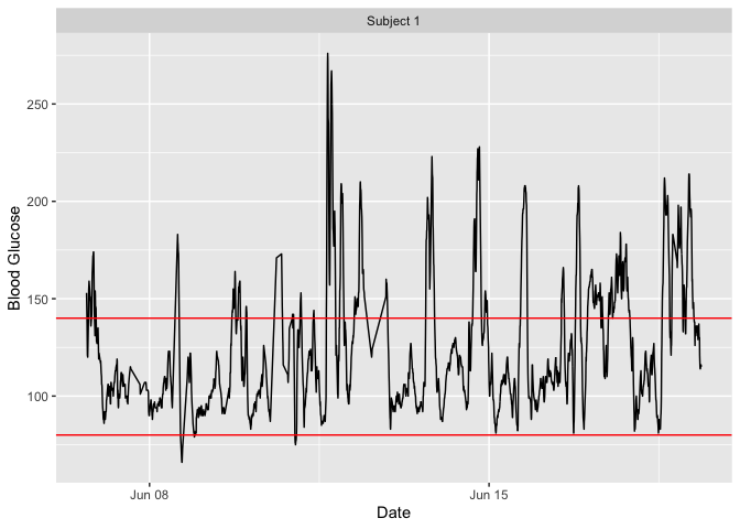
# Summary statistics and some metrics
summary_glu(example_data_1_subject)
#> # A tibble: 1 x 7
#> # Groups:   id [1]
#>   id         Min. `1st Qu.` Median  Mean `3rd Qu.`  Max.
#>   <fct>     <dbl>     <dbl>  <dbl> <dbl>     <dbl> <dbl>
#> 1 Subject 1    66        99    112  124.       143   276

in_range_percent(example_data_1_subject)
#> # A tibble: 1 x 4
#>   id        in_range_70_140 in_range_70_180 in_range_80_200
#>   <fct>               <dbl>           <dbl>           <dbl>
#> 1 Subject 1            73.7            91.7            96.0

above_percent(example_data_1_subject, targets = c(80,140,200,250))
#> # A tibble: 1 x 5
#>   id        above_140 above_200 above_250 above_80
#>   <fct>         <dbl>     <dbl>     <dbl>    <dbl>
#> 1 Subject 1      26.7      3.70     0.446     99.4

j_index(example_data_1_subject)
#> # A tibble: 1 x 2
#>   id        j_index
#>   <fct>       <dbl>
#> 1 Subject 1    24.6

conga(example_data_1_subject)
#> # A tibble: 1 x 2
#>   id        conga
#>   <fct>     <dbl>
#> 1 Subject 1  37.0

# Load multiple subject data
data(example_data_5_subject)

plot_glu(example_data_5_subject, plottype = 'lasagna', datatype = 'average')
#> Warning in CGMS2DayByDay(., tz = tz, dt0 = dt0, inter_gap = inter_gap):
#> During time conversion, 12 values were set to NA. Check the correct time zone
#> specification.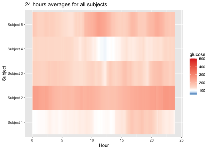
below_percent(example_data_5_subject, targets = c(80,170,260))
#> # A tibble: 5 x 4
#>   id        below_170 below_260 below_80
#>   <fct>         <dbl>     <dbl>    <dbl>
#> 1 Subject 1      89.6      99.7    0.652
#> 2 Subject 2      17.7      78.9    0
#> 3 Subject 3      73.5      96.0    0.913
#> 4 Subject 4      91.8     100      2.05
#> 5 Subject 5      55.3      90.3    1.13

mage(example_data_5_subject)
#> # A tibble: 5 x 2
#>   id         mage
#>   <fct>     <dbl>
#> 1 Subject 1  53.4
#> 2 Subject 2  78.2
#> 3 Subject 3  76.6
#> 4 Subject 4  42.9
#> 5 Subject 5 90.0For a demonstration of the package in a point and click interface, click the link below.