Post-GWAS processing functions
GWAS analyses produce an enormous amount of results, and it can be daunting to wade through them.
Many post-processing functions that GWAS analysts frequently use after conducting a standard GWAS are excellent. Rather than re-invent the wheel, GW-SEM will format its output to make it trivially easy to integrate into several common Post-GWAS processing functions. To help simplify the post-analytical processing of the analyses, we present several useful tips for collating the results into objects that can be used by other common Post GWAS processing applications.
Reading Summary Statistics into R
Since we are working with several chromosomes, typically analyzed independently and perhaps further chopped into sub-sections of chromosomes, we have several log files for each chromosome. My preference is to index the results across chromosomes using numbers, and along chromosomes using letters. Specifically, by using the snp argument in the GWAS function, it is possible to run a subset of SNP from a chromosome. For example, if there were 275,321 SNPs on Chromosome 1, 294,693 SNPs on Chromosome 2, and 212,164 SNPs on Chromosome 3, you might want to run the analyses in batches of 100,000 SNPs plus a remainder. For chromosome 1, this would mean the results for SNPs 1 to 100000 would be in fac1a.log, SNPs 100001 to 200000 would be in fac1b.log, and SNPs 200001 to 275,321 would be in fac1b.log (with similar results for the other chromosomes).
To simplify things, we can construct a list of file names for each chr with the following code, and then read them all into R in one step, as shown below:
c1  <- paste0(paste0("fac1",  letters)[1:8], ".log")
c2  <- paste0(paste0("fac2",  letters)[1:9], ".log")
c3  <- paste0(paste0("fac3",  letters)[1:7], ".log")
c4  <- paste0(paste0("fac4",  letters)[1:8], ".log")
c5  <- paste0(paste0("fac5",  letters)[1:7], ".log")
c6  <- paste0(paste0("fac6",  letters)[1:7], ".log")
c7  <- paste0(paste0("fac7",  letters)[1:6], ".log")
c8  <- paste0(paste0("fac8",  letters)[1:6], ".log")
c9  <- paste0(paste0("fac9",  letters)[1:5], ".log")
c10 <- paste0(paste0("fac10", letters)[1:5], ".log")
c11 <- paste0(paste0("fac11", letters)[1:5], ".log")
c12 <- paste0(paste0("fac12", letters)[1:5], ".log")
c13 <- paste0(paste0("fac13", letters)[1:4], ".log")
c14 <- paste0(paste0("fac14", letters)[1:4], ".log")
c15 <- paste0(paste0("fac15", letters)[1:3], ".log")
c16 <- paste0(paste0("fac16", letters)[1:3], ".log")
c17 <- paste0(paste0("fac17", letters)[1:3], ".log")
c18 <- paste0(paste0("fac18", letters)[1:3], ".log")
c19 <- paste0(paste0("fac19", letters)[1:3], ".log")
c20 <- paste0(paste0("fac20", letters)[1:2], ".log")
c21 <- paste0(paste0("fac21", letters)[1:2], ".log")
c22 <- paste0(paste0("fac22", letters)[1:2], ".log")
We can then use these object in the loadResults function so that all the data for each chromosome is loaded into a single object.
res <- loadResults(c(c1, c2, c3, c4, c5, c6, c7, c8, c9, c10,
                     c11, c12, c13, c14, c15, c16, c17, c18, c19, c20,
                     c21, c22), "snp_to_F")
At this point, we can combine the data from each chromosome into a single object, plot the data, write it to an external file, or use it as input for other post analytical GWAS analyses.
Constructing a Manhattan Plot
Manhattan plots are one of the most common methods for presenting GWAS results. While we have built a natural plotting function into GW-SEM that calls out to qqman, it is also simple to construct a Manhattan plot in qqman directly using the code below. Rather than plot the results into an graphics device, the code below constructs the plot in an external PDF document (which I find easier to work with when constructing figures for manuscripts).
# Plot the manhattan plot
png("FacManhattan.pdf", width=1500, height=750)
par(cex.lab = 2, mai = c(1, 1, .1, .1) + 0.1, bg="transparent")
manhattan(conFac, p = "P", ylim = c(0,20))
dev.off()
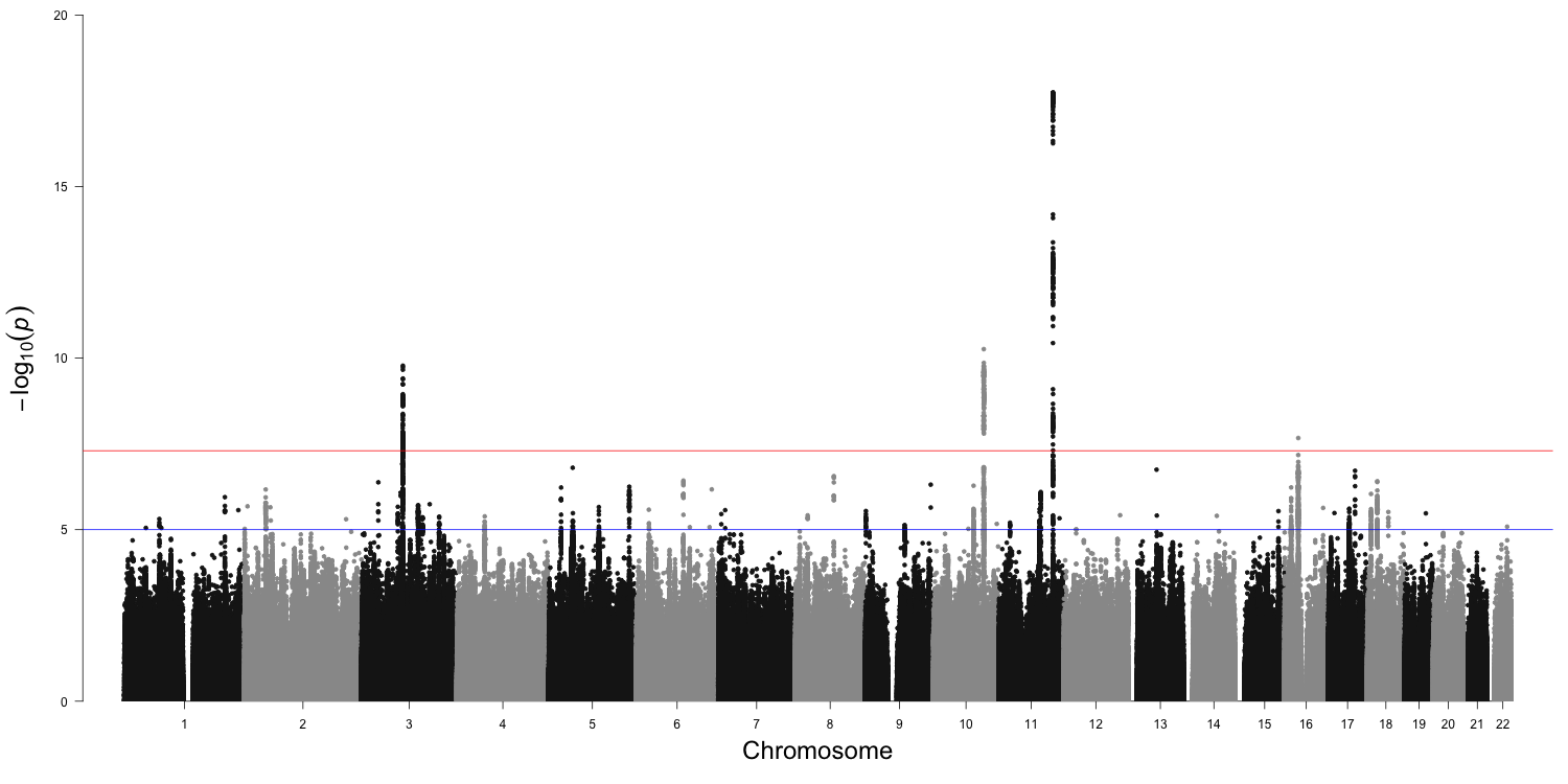
This function will produce a Manhattan plot similar to the one below:
This is the ordinal Manhattan plot from the Pritikin et al. paper for the association tests from the latent substance use frequency variable and the residuals models of substance use frequency with ordinal items for an analysis of 378,130 subjects. The x-axis presents the genomic position (Chromosomes 1–22) and the y-axis presents statistical significance as -log10p-value. The threshold for statistical significance accounting for multiple testing is shown by the red horizontal line (p = 5 × 10⁻⁸), while the blue horizontal line shows the suggestive level of statistical significance (p = 1 × 10⁻⁵).
LDhub
A common post-analytical step in many GWAS is to estimate the SNP heritability (h2snp) from the summary statistics or the genetic correlations (rg-snp) with other GWAS results. GW-SEM simplifies this process such that when summary statistics are read into R with the loadResults function, they are in the form that is required by LD Hub, or a local LD score regression analysis. All that users need to do is to write the results object to an external file.
myResults <- loadResults(c(c1, c2, c3, c4, c5, c6, c7, c8, c9, c10,
                       c11, c12, c13, c14, c15, c16, c17, c18, c19, c20,
               c21, c22), "snp_to_F")

head(myResults)
#   MxComputeLoop1 CHR    BP         SNP A1 A2 statusCode    snp_to_F  snp_to_FSE         Z         P
# 1              1   1 10177 rs367896724 AC  A         OK 0.007537512 0.008575259 0.8789837 0.3794101
# 2              2   1 10352 rs201106462 TA  T         OK 0.009997416 0.008779536 1.1387181 0.2548208
# 3              3   1 11008 rs575272151  G  C         OK 0.006097807 0.014676039 0.4154941 0.6777803
# 4              4   1 11012 rs544419019  G  C         OK 0.006097807 0.014676039 0.4154941 0.6777803
# 5              5   1 13110 rs540538026  A  G         OK 0.015765205 0.019758590 0.7978912 0.4249336
# 6              6   1 13116  rs62635286  G  T         OK 0.009840498 0.011528798 0.8535580 0.3933499

write.table(myResults, "myResults.txt", quote = F, row.names = F)
LocusZoom
Once a region of interest has been identified, it is often useful to plot the relevant SNPs in the region, along with the information about the extent of linkage disequilibrium (LD) between the lead SNP and other SNPs in the region, recombination rates in the region, and known genes that are proximate to the lead SNP. LocusZoom provides an outstanding resource to efficiently construct and annotate these plots.
# Read the results into R
myResults <- loadResults(c(c1, c2, c3, c4, c5, c6, c7, c8, c9, c10,
                       c11, c12, c13, c14, c15, c16, c17, c18, c19, c20,
               c21, c22), "snp_to_F")

# Subset the results by a specific chromosome
res3 <- myResults[myResults $CHR==3,]

# Find the basepair for the SNP(s) of interest
head(myResults[order(log10(myResults $P)),], 10)

# Generate an object with the relevant SNP +/- a flanking region (600kb in this case)
res3a <- res3[res3$BP > 85899045 - 600000 & res3$BP < 85899045 + 600000, ]

# Write the object to a file.
write.table(res3a, "res3a.txt", row.names = F, quote = F)
This will produce a file called res3a.txt in your working directory that can be directly uploaded to locusZoom to produce the desired plots.
If you have suggestions or requests for software integration, please contact us and we will see what we can do.