

![]()
R package for routing with GTFS (General Transit Feed Specification) data. See the website for full details.
To install:
To load the package and check the version:
## [1] '0.0.1'The main functions can be demonstrated with sample data included with the package from Berlin (the Verkehrverbund Berlin Brandenburg, or VBB). GTFS data are always stored as .zip files, and these sample data can be written to local storage with the function berlin_gtfs_to_zip().
berlin_gtfs_to_zip()
tempfiles <- list.files (tempdir (), full.names = TRUE)
filename <- tempfiles [grep ("vbb.zip", tempfiles)]
filename
## [1] "/tmp/Rtmpw9QswQ/vbb.zip"For normal package use, filename will specify the name of the local GTFS data stored as a single .zip file.
Given the name of a GTFS .zip file, filename, routing is as simple as the following code:
gtfs <- extract_gtfs (filename)
gtfs <- gtfs_timetable (gtfs) # A pre-processing step to speed up queries
gtfs_route (gtfs,
            from = "Schonlein",
            to = "Berlin Hauptbahnhof",
start_time = 12 * 3600 + 120) # 12:02 in seconds| route_name | trip_name | stop_name | arrival_time | departure_time |
|---|---|---|---|---|
| U8 | S+U Wittenau | U Schonleinstr. (Berlin) | 12:09:00 | 12:09:00 |
| U8 | S+U Wittenau | U Kottbusser Tor (Berlin) | 12:11:00 | 12:11:00 |
| U8 | S+U Wittenau | U Moritzplatz (Berlin) | 12:13:00 | 12:13:00 |
| U8 | S+U Wittenau | U Heinrich-Heine-Str. (Berlin) | 12:14:30 | 12:14:30 |
| U8 | S+U Wittenau | S+U Jannowitzbrucke (Berlin) | 12:15:30 | 12:15:30 |
| S3 | S Spandau Bhf | S+U Jannowitzbrucke (Berlin) | 12:20:54 | 12:21:24 |
| S3 | S Spandau Bhf | S+U Alexanderplatz Bhf (Berlin) | 12:22:54 | 12:23:42 |
| S3 | S Spandau Bhf | S Hackescher Markt (Berlin) | 12:24:54 | 12:25:24 |
| S3 | S Spandau Bhf | S+U Friedrichstr. Bhf (Berlin) | 12:26:54 | 12:27:42 |
| S3 | S Spandau Bhf | S+U Berlin Hauptbahnhof | 12:29:36 | 12:30:12 |
Isochrones from a nominated station - lines delineating the range reachable within a given time - can be extracted with the gtfs_isochrone() function, which returns a list of all stations reachable within the specified time period from the nominated station.
gtfs <- extract_gtfs (filename)
gtfs <- gtfs_timetable (gtfs) # A pre-processing step to speed up queries
x <- gtfs_isochrone (gtfs,
                     from = "Schonlein",
                     start_time = 12 * 3600 + 120,
                     end_time = 12 * 3600 + 720) # 10 minutes later
The function returns an object of class gtfs_isochrone containing sf-formatted sets of start and end points, along with all intermediate (“mid”) points, and routes. An additional item contains the non-convex (alpha) hull enclosing the routed points. This requires the packages geodist, sf, alphahull, and mapview to be installed. Isochrone objects have their own plot method:
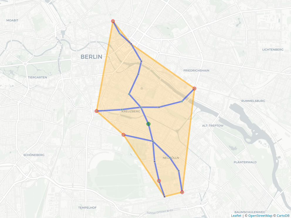
The isochrone hull also quantifies its total area and width-to-length ratio.
For background information, see gtfs.org, and particularly their GTFS Examples. The VBB is strictly schedule-only, so has no "frequencies.txt" file (this file defines “service periods”, and overrides any schedule information during the specified times).