![]()
The geometr package provides tools that generate and process easily accessible and tidy geometric shapes (of class geom). Moreover, it aims to improve interoperability of spatial and other geometric classes. Spatial classes are typically a collection of geometric shapes (or their vertices) that are accompanied by various metadata (such as attributes and a coordinate reference system). Most spatial classes are thus conceptually quite similar, yet a common standard lacks for accessing features, vertices or the metadata. Geometr fills this gap by providing tools that
or the latest development version from github:
The vignette gives an in depth introduction, explains the take on interoperability and discusses the spatial class geom that comes with geometr.
Have fun being a geometer!
Create a geom
library(geometr)
# ... from other classes
library(sf)
#> Linking to GEOS 3.5.1, GDAL 2.2.2, PROJ 4.9.2
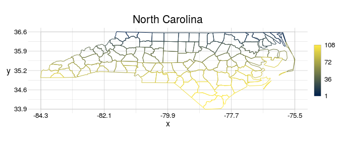
nc_sf <- st_read(system.file("shape/nc.shp", package="sf"), quiet = TRUE)
nc_geom <- gc_geom(input = nc_sf)
# ... or by hand.
library(tibble)
coords <- tibble(x = c(40, 70, 70, 50),
y = c(40, 40, 60, 70))
window <- tibble(x = c(0, 80),
y = c(0, 80))
aGeom <- gs_polygon(anchor = coords, window = window)
# The "tiny map" shows where the vertices are concentrated.
nc_geom
#> geom polygon
#> 100 groups | 108 features | 2529 points
#> crs +proj=longlat +datum=NAD27 +no_defs
#> attributes (features) AREA, PERIMETER, CNTY_, CNTY_ID, NAME, FIPS, FIPSNO, CRESS_ID, BIR74, ...
#> tiny map 36.59
#> ◌ ○ ◌ ○
#> ○ ○ ○ ○
#> ◌ ◌ ○ ◌
#> -84.32 ◌ ◌ ◌ ◌ -75.46
#> 33.88Metadata of different classes can be extracted in interoperable quality (i.e. the same metadata in different objects/classes have the same name and the same arrangement).
getFeatures(x = nc_sf)
#> Registered S3 method overwritten by 'cli':
#>   method     from
#>   print.boxx spatstat
#> # A tibble: 108 x 16
#>      fid   gid  AREA PERIMETER CNTY_ CNTY_ID NAME  FIPS  FIPSNO CRESS_ID BIR74
#>    <int> <int> <dbl>     <dbl> <dbl>   <dbl> <fct> <fct>  <dbl>    <int> <dbl>
#>  1     1     1 0.114      1.44  1825    1825 Ashe  37009  37009        5  1091
#>  2     2     2 0.061      1.23  1827    1827 Alle… 37005  37005        3   487
#>  3     3     3 0.143      1.63  1828    1828 Surry 37171  37171       86  3188
#>  4     4     4 0.07       2.97  1831    1831 Curr… 37053  37053       27   508
#>  5     5     4 0.07       2.97  1831    1831 Curr… 37053  37053       27   508
#>  6     6     4 0.07       2.97  1831    1831 Curr… 37053  37053       27   508
#>  7     7     5 0.153      2.21  1832    1832 Nort… 37131  37131       66  1421
#>  8     8     6 0.097      1.67  1833    1833 Hert… 37091  37091       46  1452
#>  9     9     7 0.062      1.55  1834    1834 Camd… 37029  37029       15   286
#> 10    10     8 0.091      1.28  1835    1835 Gates 37073  37073       37   420
#> # … with 98 more rows, and 5 more variables: SID74 <dbl>, NWBIR74 <dbl>,
#> #   BIR79 <dbl>, SID79 <dbl>, NWBIR79 <dbl>
getFeatures(x = nc_geom)
#> # A tibble: 108 x 16
#>      fid   gid  AREA PERIMETER CNTY_ CNTY_ID NAME  FIPS  FIPSNO CRESS_ID BIR74
#>    <int> <int> <dbl>     <dbl> <dbl>   <dbl> <fct> <fct>  <dbl>    <int> <dbl>
#>  1     1     1 0.114      1.44  1825    1825 Ashe  37009  37009        5  1091
#>  2     2     2 0.061      1.23  1827    1827 Alle… 37005  37005        3   487
#>  3     3     3 0.143      1.63  1828    1828 Surry 37171  37171       86  3188
#>  4     4     4 0.07       2.97  1831    1831 Curr… 37053  37053       27   508
#>  5     5     4 0.07       2.97  1831    1831 Curr… 37053  37053       27   508
#>  6     6     4 0.07       2.97  1831    1831 Curr… 37053  37053       27   508
#>  7     7     5 0.153      2.21  1832    1832 Nort… 37131  37131       66  1421
#>  8     8     6 0.097      1.67  1833    1833 Hert… 37091  37091       46  1452
#>  9     9     7 0.062      1.55  1834    1834 Camd… 37029  37029       15   286
#> 10    10     8 0.091      1.28  1835    1835 Gates 37073  37073       37   420
#> # … with 98 more rows, and 5 more variables: SID74 <dbl>, NWBIR74 <dbl>,
#> #   BIR79 <dbl>, SID79 <dbl>, NWBIR79 <dbl>
geometr only knows the feature types point, line, polygon and grid (a systematic lattice of points). In contrast to the simple features standard, there are no MULTI* features. The way simple features have been implemented in R means that the same information can be stored in several different ways, which are only interoperable after a range of tests and corrections. For example, a group of polygons can make up a MULTIPOLYGON with attributes that are valid for the overall group only. Likewise, the polygons could be stored at the level of individual “closed paths” as POLYGON, with specific attributes per polygon. Both sets of attributes can only exists either as duplicates for all group specific attributes in a POLYGON, or even more complicated nested attribute tables at the MULTIPOLYGON level.
The backbone of a geom are three attribute tables, one for points, features and groups of features, the latter two of which can be provided with ancillary information. Each feature is stored as a single unit, all of which are related to other features by a group ID, which relates the features to attributes for an overall group. Eventually this results in a tidier data-structure with easier access than Spatial* of sf objects and with higher versatility.
# when using the group = TRUE argument, the attributes of MULTI*-feature are
# stored in the group attribute table of a geom
nc_geom <- gc_geom(input = nc_sf, group = TRUE)
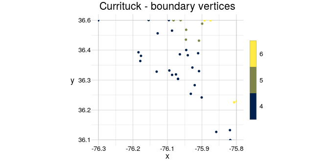
currituck <- getFeatures(x = nc_geom, gid == 4)
getFeatures(x = currituck)
#> # A tibble: 3 x 2
#> fid gid
#> <int> <int>
#> 1 4 4
#> 2 5 4
#> 3 6 4
getGroups(x = currituck)
#> # A tibble: 1 x 15
#> gid AREA PERIMETER CNTY_ CNTY_ID NAME FIPS FIPSNO CRESS_ID BIR74 SID74
#> <int> <dbl> <dbl> <dbl> <dbl> <fct> <fct> <dbl> <int> <dbl> <dbl>
#> 1 4 0.07 2.97 1831 1831 Curr… 37053 37053 27 508 1
#> # … with 4 more variables: NWBIR74 <dbl>, BIR79 <dbl>, SID79 <dbl>,
#> # NWBIR79 <dbl>
# and new attributes can be set easily,
newTable <- data.frame(fid = c(1:108),
attrib = rnorm(108))
(nc_geom <- setFeatures(x = nc_geom, table = newTable))
#> geom polygon
#> 100 groups | 108 features | 2529 points
#> crs +proj=longlat +datum=NAD27 +no_defs
#> attributes (features) attrib
#> (groups) AREA, PERIMETER, CNTY_, CNTY_ID, NAME, FIPS, FIPSNO, CRESS_ID, BIR74, ...
#> tiny map 36.59
#> ◌ ○ ◌ ○
#> ○ ○ ○ ○
#> ◌ ◌ ○ ◌
#> -84.32 ◌ ◌ ◌ ◌ -75.46
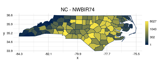
#> 33.88geometr comes with the visualise function, which makes nice-looking diagnostic spatial plots, that show explicit values whenever possible. For example, it does not create artificial bins for the values scale, but shows the explicit range of values. Moreover, you can easily set plot titles without much effort.
By default, visualise uses the feature ID as fillcolour. You can use quick options to modify which aspect given object should be shown in the plot, for example to scale the fillcolour to the attribute NWBIR74.
Each geom has the slot @window, which contains a reference window. This reference window can be used or modified in many functions of geometr
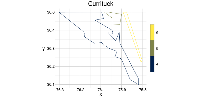
Finally, cast a geom to another type simply by providing it in anchor of the respective type
library(magrittr)
boundPoints <- gs_point(anchor = currituck) %>%
   setWindow(to = getExtent(.))
visualise(`Currituck - boundary vertices`= boundPoints, linecol = fid)