
![]()
The R package fastpos provides a fast algorithm to calculate the required sample size for a Pearson correlation to stabilize within a sequential framework (Schönbrodt & Perugini, 2013, 2018). Basically, one wants to find the sample size at which one can be sure that 1-α percent of many studies will fall into a specified corridor of stability around an assumed population correlation and stay inside that corridor if more participants are added to the study. For instance, find out how many participants per study are required so that, out of 100k studies, 90% would fall into the region between .4 to .6 (a Pearson correlation) and not leave this region again when more participants are added (under the assumption that the population correlation is .5). This sample size is also referred to as the critical point of stability for the specific parameters.
This approach is related to accuracy in parameter estimation (AIPE, e.g. Maxwell, Kelley, & Rausch, 2008) and as such can be seen as an alternative to power analysis. Unlike AIPE, the concept of stability incorporates the idea of sequentially adding participants to a study. Although the approach is young, it has already attracted a lot of interest in the psychological research community, which is evident in over 600 citations of the original publication (Schönbrodt & Perugini, 2013). To date there exists no easy way to use sequential stability for individual sample size planning because there is no analytical solution to the problem and a simulation approach is computationally expensive. The package fastpos overcomes this limitation by speeding up the calculation of correlations. For typical parameters, the theoretical speedup should be at least around 250. An empirical benchmark for a typical scenario even shows a speedup of about 400, paving the way for a wider usage of the stability approach.
You can install the released version of fastpos from CRAN with:
You can install the development version from GitHub with devtools (and vignettes build, this takes a couple of seconds longer):
If you have found this page, I assume you either want to (1) calculate the critical point of stability for your own study or (2) explore the method in general. If this is the case, read on and you should find what you are looking for. Let us first load the package and set a seed for reproducibility:
In most cases you will just need the function find_critical_pos which will give you the critical point of stability for your specific parameters.
Let us reproduce Schönbrodt and Perugini’s quite famous and oft-cited table of the critical points of stability for a precision of 0.1. We reduce the number of studies to 10k so that it runs fairly quickly.
find_critical_pos(rho = seq(.1, .7, .1), sample_size_max = 1000,
                  n_studies = 10000)
#> Warning in find_critical_pos(rho = seq(0.1, 0.7, 0.1), sample_size_max = 1000, : 37 simulation[s] did not reach the corridor of
#>             stability.
#> Increase sample_size_max and rerun the simulation.
#>   rho_pop 80%   90%    95% sample_size_min sample_size_max lower_limit upper_limit n_studies n_not_breached precision
#> 1     0.1 253 361.0 479.05              20            1000         0.0         0.2     10000             14       0.1
#> 2     0.2 237 339.0 445.00              20            1000         0.1         0.3     10000             16       0.1
#> 3     0.3 212 304.1 402.00              20            1000         0.2         0.4     10000              5       0.1
#> 4     0.4 184 261.0 346.00              20            1000         0.3         0.5     10000              1       0.1
#> 5     0.5 142 205.1 273.00              20            1000         0.4         0.6     10000              0       0.1
#> 6     0.6 103 147.0 200.00              20            1000         0.5         0.7     10000              1       0.1
#> 7     0.7  64  96.0 127.05              20            1000         0.6         0.8     10000              0       0.1
#>   precision_rel
#> 1         FALSE
#> 2         FALSE
#> 3         FALSE
#> 4         FALSE
#> 5         FALSE
#> 6         FALSE
#> 7         FALSE
The results are very close to Schönbrodt and Perugini’s table (see https://github.com/nicebread/corEvol). Note that a warning is shown, because in some simulations the corridor of stability was not reached. As long as this number is low, this should not affect the estimates much. But if you want to get more accurate estimates, then increase the maximum sample size.
If you want to dig deeper, you can have a look at the functions that find_critical_pos builds upon. simulate_pos is the workhorse of the package. It calls a C++ function to calculate correlations sequentially and it does this pretty quickly (but you know that already, right?). A rawish approach would be to create a population with create_pop and pass it to simulate_pos:
pop <- create_pop(0.5, 1000000)
pos <- simulate_pos(x_pop = pop[,1],
                    y_pop = pop[,2],
                    n_studies = 10000,
                    sample_size_min = 20,
                    sample_size_max = 1000,
                    replace = T,
                    lower_limit = 0.4,
                    upper_limit = 0.6)
hist(pos, xlim = c(0, 1000), xlab = c("Point of stability"),
     main = "Histogram of points of stability for rho = .5+-.1")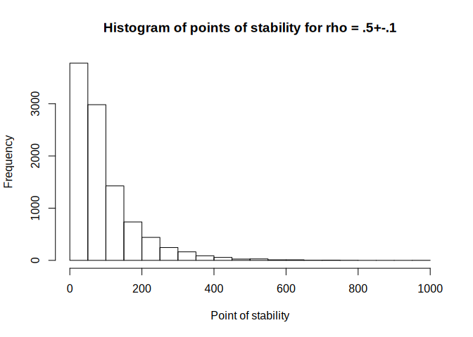
Note that no warning message appears if the corridor is not reached, but instead an NA value is returned. Pay careful attention if you work with this function, and adjust the maximum sample size as needed.
create_pop creates the population matrix by using mvrnorm. This is a much simpler way than Schönbrodt and Perugini’s approach, but the results do not seem to differ. If you are interested in how population parameters (e.g. skewness) affect the point of stability, you should instead refer to the population generating functions in Schönbrodt and Perugini’s work.
In the introduction I boldly claimed that fastpos is much faster than the original implementation of Schönbrodt and Perugini (corEvol). The theoretical argument goes as follows:
corEvol calculates every correlation from scratch. If we take the sum formula for the correlation coefficient
we can see that several sums are calculated, each consisting of adding up (the sample size) terms. This has to be done for every sample size from the minimum to the maximum one. Thus, the total number of added terms for one sum is:
On the other hand, fastpos calculates the correlation for the maximum sample size first. This requires to add numbers for one sum. Then it subtracts one value from this sum to find the correlation for the sample size , which happens repeatedly until the minimum sample size is reached. Overall the total number of terms for one sum amounts to:
The ratio between the two approaches is:
[\frac{n_{max}(n_{max}+1)/2 -(n_{min}-1)n_{min}/2}{2n_{max}-n_{min}}](https://latex.codecogs.com/png.latex?%5Cfrac%7Bn_%7Bmax%7D%28n_%7Bmax%7D%2B1%29%2F2%20-%28n_%7Bmin%7D-1%29n_%7Bmin%7D%2F2%7D%7B2n_%7Bmax%7D-n_%7Bmin%7D%7D%20 “\frac{n_{max}(n_{max}+1)/2 -(n_{min}-1)n_{min}/2}{2n_{max}-n_{min}}”)
For the typically used of 1000 and of 20, we can expect a speedup of about 250. This is only an approximation for several reasons. First, one can stop the process when the corridor is reached, which is done in fastpos but not in corEvol. Second, the main function of fastpos was written in C++ (via Rcpp), which is much faster than R. In a direct comparison between fastpos and corEvol we can expect fastpos to be at least 250 times faster.
The theoretical difference is so big that it should suffice to give a rough benchmark for which the following parameters were chosen: rho = .1, sample_size_max = 1000, sample_size_min = 20, n_studies = 10000.
Note that corEvol was written as a script for a simulation study and thus cannot be simply called via a function. Furthermore, a simulation run takes a lot of time and thus it is not practical to run it too many times. If you want to experiment with the benchmark, I have forked the original corEvol repository and made a benchmark branch (note that this will only work on GNU/Linux, since here I am using git through the bash):
git -C corEvol pull || git clone --single-branch --branch benchmark https://github.com/johannes-titz/corEvol
#> Already up to date.
For corEvol, two files are “sourced” for the benchmark. The first file generates the simulations and the second is for calculating the critical point of stability. I turned off all messages produced by these source files, except for the report of the critical point of stability—to show that it produces the same result as fastpos.
library(microbenchmark)
setwd("corEvol")
corevol <- function(){
  source("01-simdata.R")
  source("02-analyse.R")
}
bm <- microbenchmark(corevol = corevol(),
                     fastpos = find_critical_pos(rho = .1,
                                                 sample_size_max = 1000,
                                                 n_studies = 10000),
                     times = 10, unit = "s")
#> [1] "Analyzing rho = 0.1"
#>   rho 0.8_0.1 0.9_0.1 0.95_0.1
#> 1 0.1     249     355      471
#> [1] "Analyzing rho = 0.1"
#>   rho 0.8_0.1 0.9_0.1 0.95_0.1
#> 1 0.1     250     364      469
#> [1] "Analyzing rho = 0.1"
#>   rho 0.8_0.1 0.9_0.1 0.95_0.1
#> 1 0.1     249     359      471
#> [1] "Analyzing rho = 0.1"
#>   rho 0.8_0.1 0.9_0.1 0.95_0.1
#> 1 0.1     249     357      463
#> [1] "Analyzing rho = 0.1"
#>   rho 0.8_0.1 0.9_0.1 0.95_0.1
#> 1 0.1     250     364      469
#> [1] "Analyzing rho = 0.1"
#>   rho 0.8_0.1 0.9_0.1 0.95_0.1
#> 1 0.1     250     364      469
#> [1] "Analyzing rho = 0.1"
#>   rho 0.8_0.1 0.9_0.1 0.95_0.1
#> 1 0.1     253     363      475
#> [1] "Analyzing rho = 0.1"
#>   rho 0.8_0.1 0.9_0.1 0.95_0.1
#> 1 0.1     249     359      471
#> [1] "Analyzing rho = 0.1"
#>   rho 0.8_0.1 0.9_0.1 0.95_0.1
#> 1 0.1     249     359      471
#> [1] "Analyzing rho = 0.1"
#>   rho 0.8_0.1 0.9_0.1 0.95_0.1
#> 1 0.1     250     364      469
bm
#> Unit: seconds
#>     expr        min         lq      mean    median         uq        max neval
#>  corevol 604.205445 609.666951 611.74153 611.75420 613.710455 616.786979    10
#>  fastpos   1.388725   1.437223   1.53216   1.50323   1.599481   1.782225    10
For the chosen parameters, fastpos is about 400 times faster than corEvol, for which there are two main reasons: (1) fastpos is built around a C++ function via Rcpp and (2) this function does not calculate every calculation from scratch, but only calculates the difference between the correlation at sample size and via the sum formula of the Pearson correlation (see above). There are some other factors that might play a role, but they cannot account for the large difference found. For instance, setting up a population takes quite long in corEvol (about 20s), but compared to the ~9min required overall, this is only a small fraction. There are other parts of the corEvol code that are fated to be slow, but again, a speedup by a factor of 400 cannot be achieved by improving these parts. The presented benchmark is definitely not comprehensive, but only demonstrates that fastpos can be used with no significant waiting time for a typical scenario, while for corEvol this is not the case. The theoretically expected speedup by a factor of 250 was clearly exceeded.
One might think that corEvol can work with more than one core out of the box. But it is quite easy to also parallelize fastpos, for instance with mclapply from the parallel package. Furthermore, even a parallelized version of corEvol would need more than 400 cores to compete with fastpos. Overall, the speedup should be evident and will hopefully pave the way for a wider usage of the stability approach for sample size planning.
In this case fastpos will return an NA value for the point of stability. When calculating the quantiles, fastpos will use the maximum sample size, which is a more reasonable estimate than ignoring the specific simulation study altogether.
If the same parameters are used, the differences are rather small. In general, differences cannot be avoided entirely due to the random nature of the whole process. Even if the same algorithm is used, the estimates will vary slightly from run to run. The other more important aspect is how studies are treated where the point of stability is not reached: corEvol ignores them, while fastpos assumes that the corridor was reached at the maximum sample size. Thus, if the parameters are the same, fastpos will tend to produce larger estimates, which is more accurate (and more conservative). But note that if the corridor of stability is not reached, then you should increase the maximum sample size. Previously, this was not feasible due to the computational demands, but with fastpos it usually can be done.
If you find any bugs, please use the issue tracker at:
https://github.com/johannes-titz/fastpos/issues
If you need answers on how to use the package, drop me an e-mail at johannes at titz.science or johannes.titz at gmail.com
Comments and feedback of any kind are very welcome! I will thoroughly consider every suggestion on how to improve the code, the documentation, and the presented examples. Even minor things, such as suggestions for better wording or improving grammar in any part of the package, are more than welcome.
If you want to make a pull request, please check that you can still build the package without any errors, warnings, or notes. Overall, simply stick to the R packages book: https://r-pkgs.org/ and follow the code style described here: http://r-pkgs.had.co.nz/r.html#style
Maxwell, S. E., Kelley, K., & Rausch, J. R. (2008). Sample size planning for statistical power and accuracy in parameter estimation. Annual Review of Psychology, 59, 537–563. https://doi.org/10.1146/annurev.psych.59.103006.093735
Schönbrodt, F. D., & Perugini, M. (2013). At what sample size do correlations stabilize? Journal of Research in Personality, 47, 609–612. https://doi.org/10.1016/j.jrp.2013.05.009
Schönbrodt, F. D., & Perugini, M. (2018). Corrigendum to “At What Sample Size Do Correlations Stabilize?” [J. Res. Pers. 47 (2013) 609–612]. Journal of Research in Personality, 74, 194. https://doi.org/10.1016/j.jrp.2018.02.010