

diffeqr is a package for solving differential equations in R. It utilizes DifferentialEquations.jl for its core routines to give high performance solving of ordinary differential equations (ODEs), stochastic differential equations (SDEs), delay differential equations (DDEs), and differential-algebraic equations (DAEs) directly in R.
If you have any questions, or just want to chat about solvers/using the package, please feel free to chat in the Gitter channel. For bug reports, feature requests, etc., please submit an issue.
diffeqr is registered into CRAN. Thus to use add the package, use:
To install the master branch of the package (for developers), use:
You will need a working installation of Julia in your path. To install Julia, download a generic binary from the JuliaLang site and add it to your path. The download and installation of DifferentialEquations.jl will happen on the first invocation of diffeqr::diffeq_setup().
diffeqr does not provide the full functionality of DifferentialEquations.jl. Instead, it supplies simplified direct solving routines with an R interface. The most basic function is:
which solves the ODE u' = f(u,p,t) where u(0)=u0 over the timespan tspan. The common interface arguments are documented at the DifferentialEquations.jl page. Notice that not all options are allowed, but the most common arguments are supported.
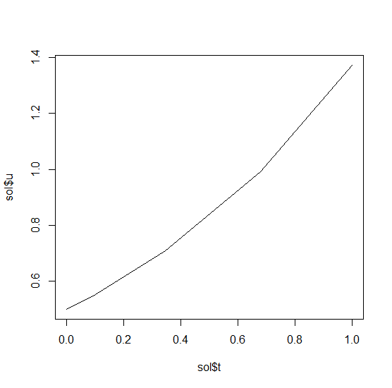
Let’s solve the linear ODE u'=1.01u. First setup the package:
Define the derivative function f(u,p,t).
Then we give it an initial condition and a time span to solve over:
With those pieces we call diffeqr::ode.solve to solve the ODE:
This gives back a solution object for which sol$t are the time points and sol$u are the values. We can check it by plotting the solution:
Now let’s solve the Lorenz equations. In this case, our initial condition is a vector and our derivative functions takes in the vector to return a vector (note: arbitrary dimensional arrays are allowed). We would define this as:
f <- function(u,p,t) {
du1 = p[1]*(u[2]-u[1])
du2 = u[1]*(p[2]-u[3]) - u[2]
du3 = u[1]*u[2] - p[3]*u[3]
return(c(du1,du2,du3))
}Here we utilized the parameter array p. Thus we use diffeqr::ode.solve like before, but also pass in parameters this time:
u0 = c(1.0,0.0,0.0)
tspan <- list(0.0,100.0)
p = c(10.0,28.0,8/3)
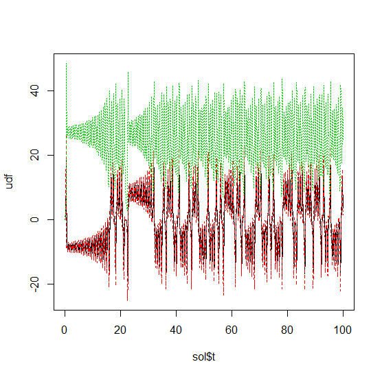
sol = diffeqr::ode.solve(f,u0,tspan,p=p)The returned solution is like before. It is convenient to turn it into a data.frame:
Now we can use matplot to plot the timeseries together:
Now we can use the Plotly package to draw a phase plot:
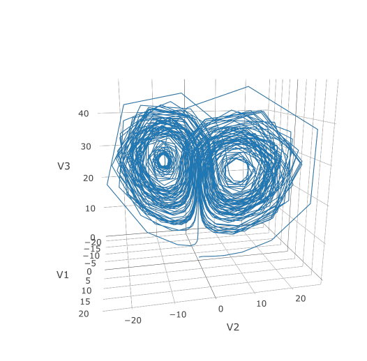
Plotly is much prettier!
If we want to have a more accurate solution, we can send abstol and reltol. Defaults are 1e-6 and 1e-3 respectively. Generally you can think of the digits of accuracy as related to 1 plus the exponent of the relative tolerance, so the default is two digits of accuracy. Absolute tolernace is the accuracy near 0.
In addition, we may want to choose to save at more time points. We do this by giving an array of values to save at as saveat. Together, this looks like:
abstol = 1e-8
reltol = 1e-8
saveat = 0:10000/100
sol = diffeqr::ode.solve(f,u0,tspan,p=p,abstol=abstol,reltol=reltol,saveat=saveat)
udf = as.data.frame(sol$u)
plotly::plot_ly(udf, x = ~V1, y = ~V2, z = ~V3, type = 'scatter3d', mode = 'lines')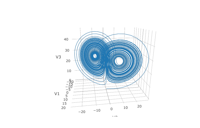
We can also choose to use a different algorithm. The choice is done using a string that matches the Julia syntax. See the ODE tutorial for details. The list of choices for ODEs can be found at the ODE Solvers page. For example, let’s use a 9th order method due to Verner:
Note that each algorithm choice will cause a JIT compilation.
One way to enhance the performance of your code is to define the function in Julia so that way it is JIT compiled. diffeqr is built using the JuliaCall package, and so you can utilize this same interface to define a function directly in Julia:
f <- JuliaCall::julia_eval("
function f(du,u,p,t)
du[1] = 10.0*(u[2]-u[1])
du[2] = u[1]*(28.0-u[3]) - u[2]
du[3] = u[1]*u[2] - (8/3)*u[3]
end")We can then use this in our ODE function by telling it to use the Julia-defined function called f:
This will help a lot if you are solving difficult equations (ex. large PDEs) or repeat solving (ex. parameter estimation).
Solving stochastic differential equations (SDEs) is the similar to ODEs. To solve an SDE, you use diffeqr::sde.solve and give two functions: f and g, where du = f(u,t)dt + g(u,t)dW_t
f <- function(u,p,t) {
  return(1.01*u)
}
g <- function(u,p,t) {
return(0.87*u)
}
u0 = 1/2
tspan <- list(0.0,1.0)
sol = diffeqr::sde.solve(f,g,u0,tspan)
plotly::plot_ly(udf, x = sol$t, y = sol$u, type = 'scatter', mode = 'lines')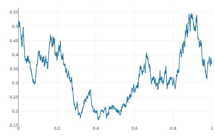
Let’s add diagonal multiplicative noise to the Lorenz attractor. diffeqr defaults to diagonal noise when a system of equations is given. This is a unique noise term per system variable. Thus we generalize our previous functions as follows:
f <- function(u,p,t) {
  du1 = p[1]*(u[2]-u[1])
  du2 = u[1]*(p[2]-u[3]) - u[2]
  du3 = u[1]*u[2] - p[3]*u[3]
  return(c(du1,du2,du3))
}
g <- function(u,p,t) {
return(c(0.3*u[1],0.3*u[2],0.3*u[3]))
}
u0 = c(1.0,0.0,0.0)
tspan <- list(0.0,1.0)
p = c(10.0,28.0,8/3)
sol = diffeqr::sde.solve(f,g,u0,tspan,p=p,saveat=0.005)
udf = as.data.frame(sol$u)
plotly::plot_ly(x = sol$t, y = sol$u, type = 'scatter', mode = 'lines')Using a JIT compiled function for the drift and diffusion functions can greatly enhance the speed here. With the speed increase we can comfortably solve over long time spans:
f <- JuliaCall::julia_eval("
function f(du,u,p,t)
  du[1] = 10.0*(u[2]-u[1])
  du[2] = u[1]*(28.0-u[3]) - u[2]
  du[3] = u[1]*u[2] - (8/3)*u[3]
end")
g <- JuliaCall::julia_eval("
function g(du,u,p,t)
du[1] = 0.3*u[1]
du[2] = 0.3*u[2]
du[3] = 0.3*u[3]
end")
tspan <- list(0.0,100.0)
sol = diffeqr::sde.solve('f','g',u0,tspan,p=p,saveat=0.05)
udf = as.data.frame(sol$u)
#plotly::plot_ly(udf, x = ~V1, y = ~V2, z = ~V3, type = 'scatter3d', mode = 'lines')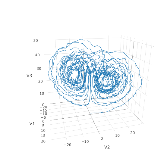
In many cases you may want to share noise terms across the system. This is known as non-diagonal noise. The DifferentialEquations.jl SDE Tutorial explains how the matrix form of the diffusion term corresponds to the summation style of multiple Wiener processes. Essentially, the row corresponds to which system the term is applied to, and the column is which noise term. So du[i,j] is the amount of noise due to the jth Wiener process that’s applied to u[i]. We solve the Lorenz system with correlated noise as follows:
f <- JuliaCall::julia_eval("
function f(du,u,p,t)
  du[1] = 10.0*(u[2]-u[1])
  du[2] = u[1]*(28.0-u[3]) - u[2]
  du[3] = u[1]*u[2] - (8/3)*u[3]
end")
g <- JuliaCall::julia_eval("
function g(du,u,p,t)
  du[1,1] = 0.3u[1]
  du[2,1] = 0.6u[1]
  du[3,1] = 0.2u[1]
  du[1,2] = 1.2u[2]
  du[2,2] = 0.2u[2]
  du[3,2] = 0.3u[2]
end")
u0 = c(1.0,0.0,0.0)
tspan <- list(0.0,100.0)
noise.dims = list(3,2)
sol = diffeqr::sde.solve('f','g',u0,tspan,saveat=0.005,noise.dims=noise.dims)
udf = as.data.frame(sol$u)
plotly::plot_ly(udf, x = ~V1, y = ~V2, z = ~V3, type = 'scatter3d', mode = 'lines')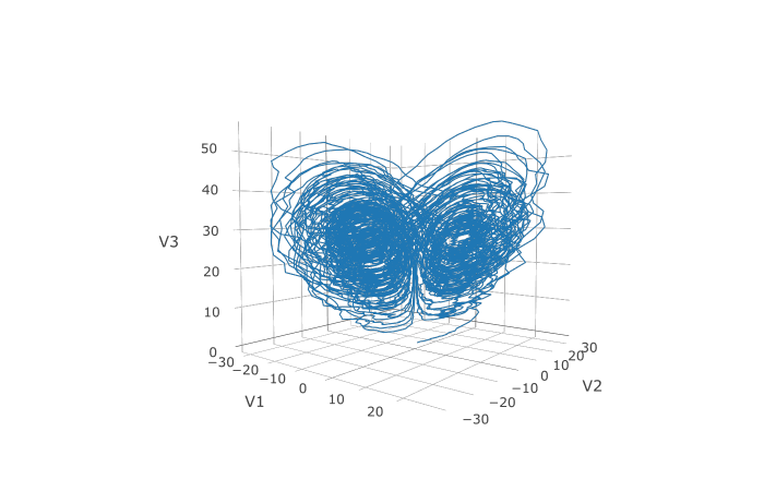
Here you can see that the warping effect of the noise correlations is quite visible!
A differential-algebraic equation is defined by an implicit function f(du,u,p,t)=0. All of the controls are the same as the other examples, except here you define a function which returns the residuals for each part of the equation to define the DAE. The initial value u0 and the initial derivative du0 are required, though they do not necessarily have to satisfy f (known as inconsistant initial conditions). The methods will automatically find consistant initial conditions. In order for this to occur, differential_vars must be set. This vector states which of the variables are differential (have a derivative term), with false meaning that the variable is purely algebraic.
This example shows how to solve the Robertson equation:
f <- function (du,u,p,t) {
  resid1 = - 0.04*u[1]              + 1e4*u[2]*u[3] - du[1]
  resid2 = + 0.04*u[1] - 3e7*u[2]^2 - 1e4*u[2]*u[3] - du[2]
  resid3 = u[1] + u[2] + u[3] - 1.0
  c(resid1,resid2,resid3)
}
u0 = c(1.0, 0, 0)
du0 = c(-0.04, 0.04, 0.0)
tspan = list(0.0,100000.0)
differential_vars = c(TRUE,TRUE,FALSE)
sol = diffeqr::dae.solve(f,du0,u0,tspan,differential_vars=differential_vars)
udf = as.data.frame(sol$u)
plotly::plot_ly(udf, x = sol$t, y = ~V1, type = 'scatter', mode = 'lines') %>%
plotly::add_trace(y = ~V2) %>%
plotly::add_trace(y = ~V3)
Additionally, an in-place JIT compiled form for f can be used to enhance the speed:
f = JuliaCall::julia_eval("function f(out,du,u,p,t)
  out[1] = - 0.04u[1]              + 1e4*u[2]*u[3] - du[1]
  out[2] = + 0.04u[1] - 3e7*u[2]^2 - 1e4*u[2]*u[3] - du[2]
  out[3] = u[1] + u[2] + u[3] - 1.0
end")
sol = diffeqr::dae.solve('f',du0,u0,tspan,differential_vars=differential_vars)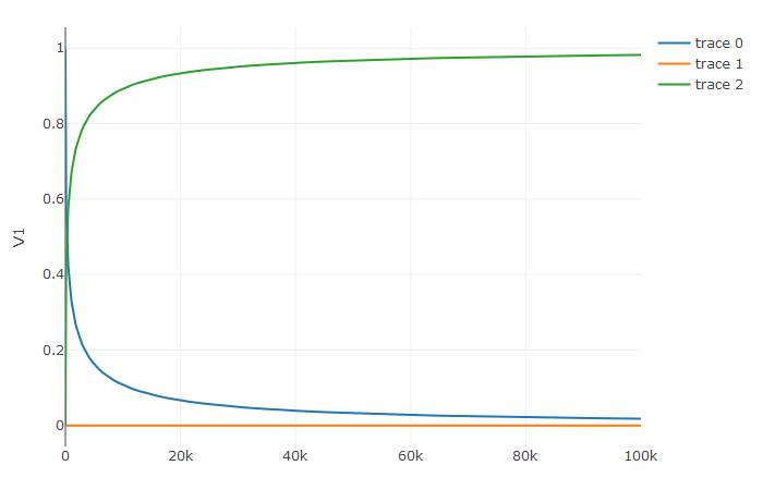
A delay differential equation is an ODE which allows the use of previous values. In this case, the function needs to be a JIT compiled Julia function. It looks just like the ODE, except in this case there is a function h(p,t) which allows you to interpolate and grab previous values.
We must provide a history function h(p,t) that gives values for u before t0. Here we assume that the solution was constant before the initial time point. Additionally, we pass constant_lags = c(20.0) to tell the solver that only constant-time lags were used and what the lag length was. This helps improve the solver accuracy by accurately stepping at the points of discontinuity. Together this is:
f = JuliaCall::julia_eval("function f(du, u, h, p, t)
  du[1] = 1.1/(1 + sqrt(10)*(h(p, t-20)[1])^(5/4)) - 10*u[1]/(1 + 40*u[2])
  du[2] = 100*u[1]/(1 + 40*u[2]) - 2.43*u[2]
end")
u0 = c(1.05767027/3, 1.030713491/3)
h <- function (p,t){
  c(1.05767027/3, 1.030713491/3)
}
tspan = list(0.0, 100.0)
constant_lags = c(20.0)
sol = diffeqr::dde.solve('f',u0,h,tspan,constant_lags=constant_lags)
udf = as.data.frame(sol$u)
plotly::plot_ly(udf, x = sol$t, y = ~V1, type = 'scatter', mode = 'lines') %>% plotly::add_trace(y = ~V2)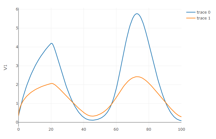
Notice that the solver accurately is able to simulate the kink (discontinuity) at t=20 due to the discontinuity of the derivative at the initial time point! This is why declaring discontinuities can enhance the solver accuracy.