did

The package contains tools for computing average treatment effect parameters in Difference in Differences models with more than two periods, with variation in treatment timing across individuals, and where the DID assumption possibly holds conditional on covariates. The main parameters are group-time average treatment effects which are the average treatment effect for a particular group at a a particular time. These can be aggregated into a fewer number of treatment effect parameters, and the package deals with the cases where there is selective treatment timing, dynamic treatment effects, calendar time effects, or combinations of these. There are also functions for testing the Difference in Differences assumption, and plotting group-time average treatment effects.

Installation

You can install from CRAN with:

install.packages("did")

or get the latest version from github with:

# install.packages("devtools")
devtools::install_github("bcallaway11/did")

Example

The following is a simplified example of the effect of states increasing their minimum wages on county-level teen employment rates which comes from Callaway and Sant’Anna (2019).

A subset of the data is available in the package and can be loaded by

  library(did)
  data(mpdta)

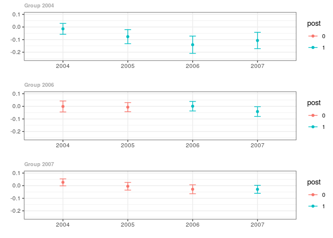
The dataset contains 500 observations of county-level teen employment rates from 2003-2007. Some states are first treated in 2004, some in 2006, and some in 2007 (see the paper for details). We are interested in estimating the group-time average treatment effect, which is the average treatment effect in period (t) for the group of states first treated in period (g) and given by \[\begin{align*} ATT(g,t)=E[Y_t(1) - Y_t(0)|G_g=1] \end{align*}\] under the common trends assumption: \[\begin{align*} E[\Delta Y_t(0) | X, G_g=1] = E[\Delta Y_t(0) | X, C=1] \ a.s. \quad \forall g\leq t \end{align*}\] where (Y_t(1)) and (Y_t(0)) denote treated and untreated potential outcomes, (G_g=1) denotes counties first treated in period (g), (C=1) denotes control counties that are never treated.

To estimate (ATT(g,t)), one can use the method as follows:

out <- mp.spatt(lemp ~ treat, xformla=~lpop, data=mpdta,
                 panel=TRUE, first.treat.name="first.treat",
                 idname="countyreal", tname="year",
                 bstrap=FALSE, se=TRUE, cband=FALSE)
#> current period: 2004 
#> current group: 2004 
#> set pretreatment period to be 2003 
#> current period: 2005 
#> current group: 2004 
#> set pretreatment period to be 2003 
#> current period: 2006 
#> current group: 2004 
#> set pretreatment period to be 2003 
#> current period: 2007 
#> current group: 2004 
#> set pretreatment period to be 2003 
#> current period: 2006 
#> current group: 2006 
#> set pretreatment period to be 2005 
#> current period: 2007 
#> current group: 2006 
#> set pretreatment period to be 2005 
#> current period: 2007 
#> current group: 2007 
#> set pretreatment period to be 2006
summary(out)
#> 
#> Reference: Callaway, Brantly and Sant'Anna, Pedro.  "Difference-in-Differences with Multiple Time Periods." Working Paper <https://ssrn.com/abstract=3148250>, 2019. 
#> 
#> 
#> 
#>  group   time          att          se
#> ------  -----  -----------  ----------
#>   2004   2004   -0.0145484   0.0219886
#>   2004   2005   -0.0764499   0.0284761
#>   2004   2006   -0.1404646   0.0350339
#>   2004   2007   -0.1069326   0.0330405
#>   2006   2004   -0.0008686   0.0221298
#>   2006   2005   -0.0063972   0.0185132
#>   2006   2006    0.0012080   0.0192254
#>   2006   2007   -0.0413082   0.0196941
#>   2007   2004    0.0265561   0.0141314
#>   2007   2005   -0.0046609   0.0155829
#>   2007   2006   -0.0283403   0.0181435
#>   2007   2007   -0.0288948   0.0162974
#> 
#> 
#> P-value for pre-test of DID assumption:  0.23803

and plot the results using the command:

library(gridExtra)
ggdid(out, ylim=c(-.25,.1))

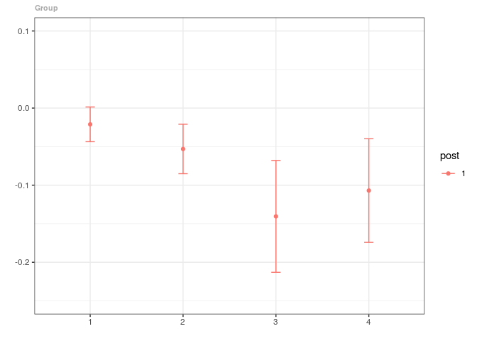
Another common use for the did package is reporting “event-study” type results. To get these directly, one can use

summary(out$aggte, type="dynamic")
#> 
#> Reference: Callaway, Brantly and Sant'Anna, Pedro.  "Difference-in-Differences with Multiple Time Periods." Working Paper <https://ssrn.com/abstract=3148250>, 2019. 
#> Overall Summary Measures 
#> ------------------------ 
#> Simple ATT    :  -0.04177708 
#>   SE          :  0.01118622 
#> Selective ATT :  -0.03287537 
#>   SE          :  0.01118622 
#> Dynamic ATT   :  -0.08037689 
#>   SE          :  0.02076471 
#> Calendar ATT  :  -0.0441701 
#>   SE          :  0.01892826 
#> 
#> Dynamic Treatment Effects 
#> -------------------------
#> 
#>   e          att          se
#> ---  -----------  ----------
#>   1   -0.0210883   0.0114816
#>   2   -0.0530221   0.0163636
#>   3   -0.1404646   0.0370100
#>   4   -0.1069326   0.0342974

and to plot the same results

ggdid(out, type="dynamic", ylim=c(-.25,.1))

Other options for both summary and ggdid are:

• “selective” – results when there is selective treatment timing

• “calendar” – results when there are calendar time effects

• “dynsel” – results when there is selective treatment timing and dynamic treatment effects; this also requires specifying the additional parameter e1 which is the required number of post-treatment periods that a group needs to experience before they are included in the sample

See the discussion in our paper for many more details:

Callaway, Brantly and Sant’Anna, Pedro. “Difference-in-Differences with Multiple Time Periods.” Working Paper https://ssrn.com/abstract=3148250, 2019.

Finally, a few things that we are working on:

• improving the vignette that goes along with the package

• event-study plots that include pre-treatment periods as well

• uniform confidence bands for event-studies (as well as other aggregated parameters)