cyanoFilter

cyaoFilter is a package designed to identify, assign indicators and/or filter out synechoccus type cyanobacteria from a water sample examined with flowcytometry.

Installation and Dependencies

Run the code below to install the package and all its dependencies.

install.packages("cyanoFilter")

All dependencies both on CRAN and bioconductor should be installed when you install the package itself. However, do install the following needed bioconductor packages should you run into errors while attempting to use the functions in this package.

install.packages("BiocManager")
library(BiocManager)
install(c("Biobase", "flowCore", "flowDensity"))

Motivation and Background

Flow cytometry (FCM) is a well-known technique for identifying cell populations in fluids. It is largely applied in biological and medical sciences for cell sorting, counting, biomarker detections and protein engineering. Identifying cell populations in flow cytometry data, a process termed gating can either be done mnually or via automated algorithms. Recenntly, researchers also apply machine learning tools to identify the different cell populations present in FCM data. Manual gating can be quite subjective and often not reproducible, but it aids the use of expert knowledge in the gating process, while machine learning tools and automated algorithms often don’t allow the use of expert knowledge in the gating process. To address this issue for cyanobacteria FCM experiments, we develop the cyanoFilter framework in R. We also demonstrate its use in filtering out two cyanobacteria strains named BS4 and BS5.

Usage

The package comes with 2 internal datasets that we use for demonstrating the usage of the functions contained in the package. The meta data file contains BS4 and BS5 samples measured with a guava easyCyte HT series at 3 dilution levels (2000, 10000 and 20000) each. The FCS file contains the flow cytometer channel measurements for one of these sample.

Meta File Preprocessing

The Good Measurements

The goodfcs() is deigned to check the (cell/)L of the meta file (normally csv) obtained from the flow cytometer and decide if the measurements in the FCS file can be trusted. This function is essentially useful for flow cytometers that are not equipped to perform automated dilution.

library(flowCore)
library(cyanoFilter)
#internally contained datafile in cyanoFilter
metadata <- system.file("extdata", "2019-03-25_Rstarted.csv", 
  package = "cyanoFilter", 
  mustWork = TRUE)
metafile <- read.csv(metadata, skip = 7, stringsAsFactors = FALSE, 
  check.names = TRUE)
#columns containing dilution, $\mu l$ and id information
metafile <- metafile[, c(1:3, 6:8)] 
knitr::kable(metafile) 

Each row in the csv file corresponds to a measurement from two types of cyanobacteria cells carried out at one of three dilution levels. The columns contain information about the dilution level, the number of cells per micro-litre ((cell/l)), number of particles measured and a unique identification code for each measurement. The Sample.ID column is structured in the format cyanobacteria_dilution. We extract the cyanobacteria part of this column into a new column and also rename the (cell/l) column with the following code:

#extract the part of the Sample.ID that corresponds to BS4 or BS5
metafile$Sample.ID2 <- stringr::str_extract(metafile$Sample.ID, "BS*[4-5]")
#clean up the Cells.muL column
names(metafile)[which(stringr::str_detect(names(metafile), "Cells."))] <- "CellspML"

The Good Measurements

To determine the appropriate data file to read from a FCM datafile, the desired minimum, maximum and column containing the (celll) values are supplied to the goodfcs() function. The code below demonstrates the use of this function for a situation where the desired minimum and maximum for (cell/l) is 50 and 1000 respectively.

metafile$Status <- cyanoFilter::goodfcs(metafile = metafile, col_cpml = "CellspML", 
                                        mxd_cellpML = 1000, mnd_cellpML = 50)

knitr::kable(metafile)

The function adds an extra column, Status, with entries good or bad to the metafile. Rows containing (cell/l) values outside the desired minimum and maximum are labelled bad. Note that the Status column for the fourth row is labelled bad, because it has a (cell/l) value outside the desired range.

Files to Retain

Although any of the files labelled good can be read from the FCM file, the retain() function can help select either the file with the highest (cell/l) or that with the smallest (cell/l) value. To do this, one supplies the function with the status column, (cell/l) column and the desired decision. The code below demonstrates this action for a case where we want to select the file with the maximum (cell/l) from the good measurements for each unique sample ID.

broken <- metafile %>% group_by(Sample.ID2) %>% nest()
metafile$Retained <- unlist(map(broken$data, function(.x) {
  retain(meta_files = .x, make_decision = "maxi",
  Status = "Status",
  CellspML = "CellspML")
 })
)
knitr::kable(metafile)

This function adds another column, Retained, to the metafile. The third and sixth row in the metadata are with the highest (cell/l) values, thus one can proceed to read the fourth and sixth file from the corresponding FCM datafile for BS4 and BS5 respectively. This implies that we are reading in only two FCM files rather than six needed files.

Flow Cytometer File Processing

To input the B4_18_1.fcs file into R, we use the read.FCS() function from the flowCore package. The dataset option enables the specification of the precise file to be read. Since this datafile contains one file only, we set this option to 1. If this option is set to 2, it gives an error since text.fcs contains only one datafile.

flowfile_path <- system.file("extdata", "B4_18_1.fcs", package = "cyanoFilter",
  mustWork = TRUE)
flowfile <- read.FCS(flowfile_path, alter.names = TRUE,
  transformation = FALSE, emptyValue = FALSE,
  dataset = 1)
flowfile
> flowFrame object ' B4_18_1'
> with 8729 cells and 11 observables:
>            name                                desc range    minRange
> $P1    FSC.HLin          Forward Scatter (FSC-HLin) 1e+05    0.000000
> $P2    SSC.HLin             Side Scatter (SSC-HLin) 1e+05  -34.479282
> $P3  GRN.B.HLin   Green-B Fluorescence (GRN-B-HLin) 1e+05  -21.194536
> $P4  YEL.B.HLin  Yellow-B Fluorescence (YEL-B-HLin) 1e+05  -10.327441
> $P5  RED.B.HLin     Red-B Fluorescence (RED-B-HLin) 1e+05   -5.347203
> $P6  NIR.B.HLin Near IR-B Fluorescence (NIR-B-HLin) 1e+05   -4.307983
> $P7  RED.R.HLin     Red-R Fluorescence (RED-R-HLin) 1e+05  -25.490185
> $P8  NIR.R.HLin Near IR-R Fluorescence (NIR-R-HLin) 1e+05  -16.020023
> $P9    SSC.ALin        Side Scatter Area (SSC-ALin) 1e+05    0.000000
> $P10      SSC.W          Side Scatter Width (SSC-W) 1e+05 -111.000000
> $P11       TIME                                Time 1e+05    0.000000
>      maxRange
> $P1     99999
> $P2     99999
> $P3     99999
> $P4     99999
> $P5     99999
> $P6     99999
> $P7     99999
> $P8     99999
> $P9     99999
> $P10    99999
> $P11    99999
> 368 keywords are stored in the 'description' slot

The R object flowfile contains measurements about cells across 10 channels since the time channel does not contain any information about the properties of the measured cells.

Transformation and visualisation

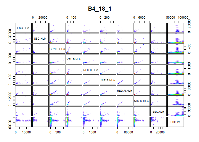
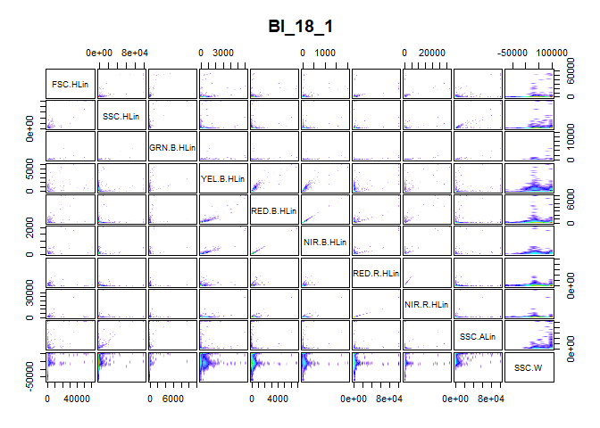
To examine the need for transformation, a visual representation of the information in the expression matrix is of great use. The pair_plot() function produces a panel plot of all measured channels. Each plot is also smoothed to show the cell density at every part of the plot.

flowfile_nona <- nona(x = flowfile)
pair_plot(flowfile_nona, notToPlot = "TIME")

We obtain Figure above by using the pair_plot() function after removing all NA values from the expression matrix with the nona() function.

#natural logarithm transformation
flowfile_noneg <- noneg(x = flowfile_nona)
flowfile_logtrans <- lnTrans(x = flowfile_noneg, 
  notToTransform = c("SSC.W", "TIME"))
pair_plot(flowfile_logtrans, notToPlot = "TIME")

The second figure is the result of performing a logarithmic transformation in addition to the previous actions taken. The logarithmic transformation appears satisfactory in this case, as it allow a better examination of the information contained in each panel of the figure. Moreover, the clusters are clearly visible in this figure compared to the former figure. Other possible transformation (linear, bi-exponential and arcsinh) can be pursued if the logarithm transformation is not satisfactory. Functions for these transformations are provided in the flowCore package.

Gating

Flow cytometry outcomes can be divided into 3 and they are not entirely mutually exclusive but this is normally not a problem as scientists are normally interested in a pre-defined outcome.

• Margin Events are particles too big to be measured
• Doublets are cells with disproportionate Area, Height relationship
• Singlets are the ‘normal cells’ but these could either be dead cells/particles (debris) and living (good cells).

The set of functions below identifies margin events and singlets. Doublets are normally pre-filtered during the event acquiring phase of measuring.

Gating margin events

To remove margin events, the cellmargin() function takes the column in the expression matrix corresponding to measurements about the width of each cell. The code below demonstrates the removal of margin events using the SSC.W column with the option to estimate the cut point between the margin events and the good cells.

flowfile_marginout <- cellmargin(flow.frame = flowfile_logtrans,
  Channel = 'SSC.W', type = 'estimate', y_toplot = "FSC.HLin")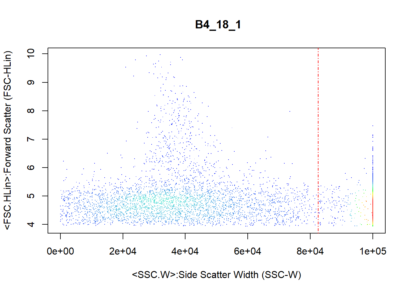

The function returns a figure (Figure @ref(fig:marginEvents)) in this case) and a list containing:

• fullflowframe, flowframe with indicator for margin and non-margin events in the expression matrix,
• reducedflowframe, flowframe containing only non-margin events
• N_margin, number of margin events contained in the input flowframe
• N_nonmargin, number of non-margin events
• N_particle, number of particles in the input flowframe

The code below accesses the number of margin and non-margin particles.

flowfile_marginout$N_margin
> [1] 3092
flowfile_marginout$N_nonmargin
> [1] 3831

Gating debris and cyanobacteria

We conceptualized the division of cells into clusters in two ways in cyanoFilter and this is reflected in two main functions that perform the clustering exercise; celldebris_nc() and celldebris_emclustering(). The celldebris_nc() function employs minimum intersection points between peaks observed in a two dimensional kernel density, while celldebris_emclustering() employs a finite mixture of multivariate normals to assign probability of belonging to a cluster to each measured particle. Both functions produce plots by default to enable users examine the results of the clustering.

After removing margin events, it is of interest to identify BS4 cyanobacteria cells contained in the text.fcs datafile that we have pre-processed until now. The following code separates BS4 cyanobacteria cells using the two channels measuring the presence of chlorophyll a, RED.B.HLin, and phycoerythrin, YEL.B.HLin. We use the knowledge of knowing that the BS4 cells will be on the right part of the RED.B.HLin channel because of the presence of chlorophyll a, and also on the lower part of the YEL.B.HLin channel due to low presence of phycoerythrin.

bs4_gate1 <- celldebris_nc(flowfile_marginout$reducedflowframe, 
  channel1 = "RED.B.HLin", channel2 = "YEL.B.HLin", 
  interest = "bottom-right", to_retain = "refined" )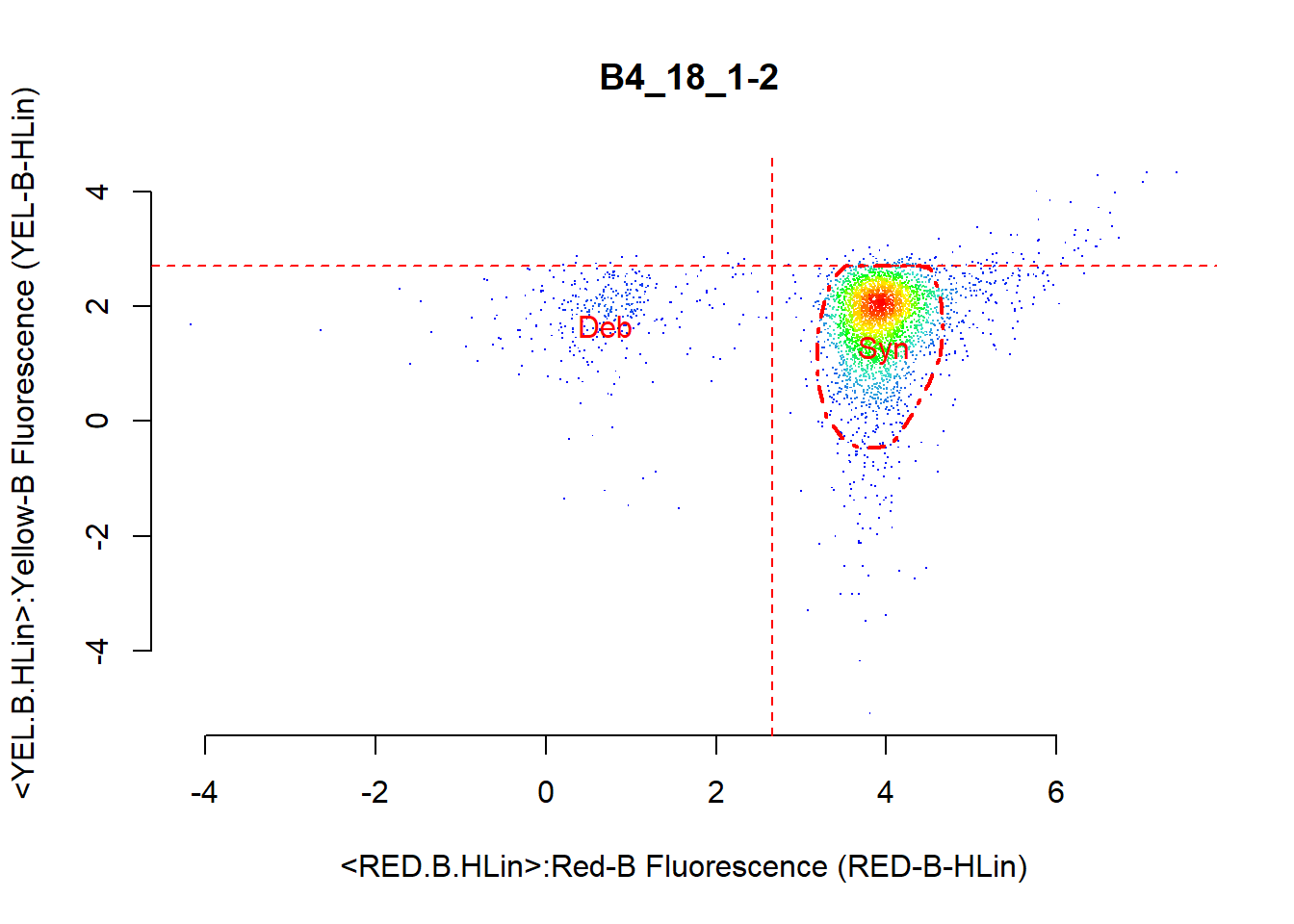

The resulting object is a figure (Figure @ref(fig:kdapproach)) and a list containing the following:

• reducedframe, a flowFrame with all debris removed
• fullframe, flowFrame with all measured particles and indicator for debris and cyanobacteria cells
• Cell_count, the number of BS4 cells counted
• Debris_Count, the number of debris particles.

An alternative function for identifying BS4 cells is the celldebris_emclustering() function. This function tries to identify the number of clusters supplied via the ncluster option, but this number is reduced if there are clusters with no particles during the EM iterations. The function can also accept more than two channels as input. The code below demonstrates its use with four channels measuring chlorophyll a, phycoerythrin, height and phycocyanin respectively.

bs4_gate2 <- celldebris_emclustering(flowfile_marginout$reducedflowframe, 
  channels =  c("RED.B.HLin", "YEL.B.HLin", "FSC.HLin", "RED.R.HLin"), 
  ncluster = 3, min.itera = 20, classifier = 0.8)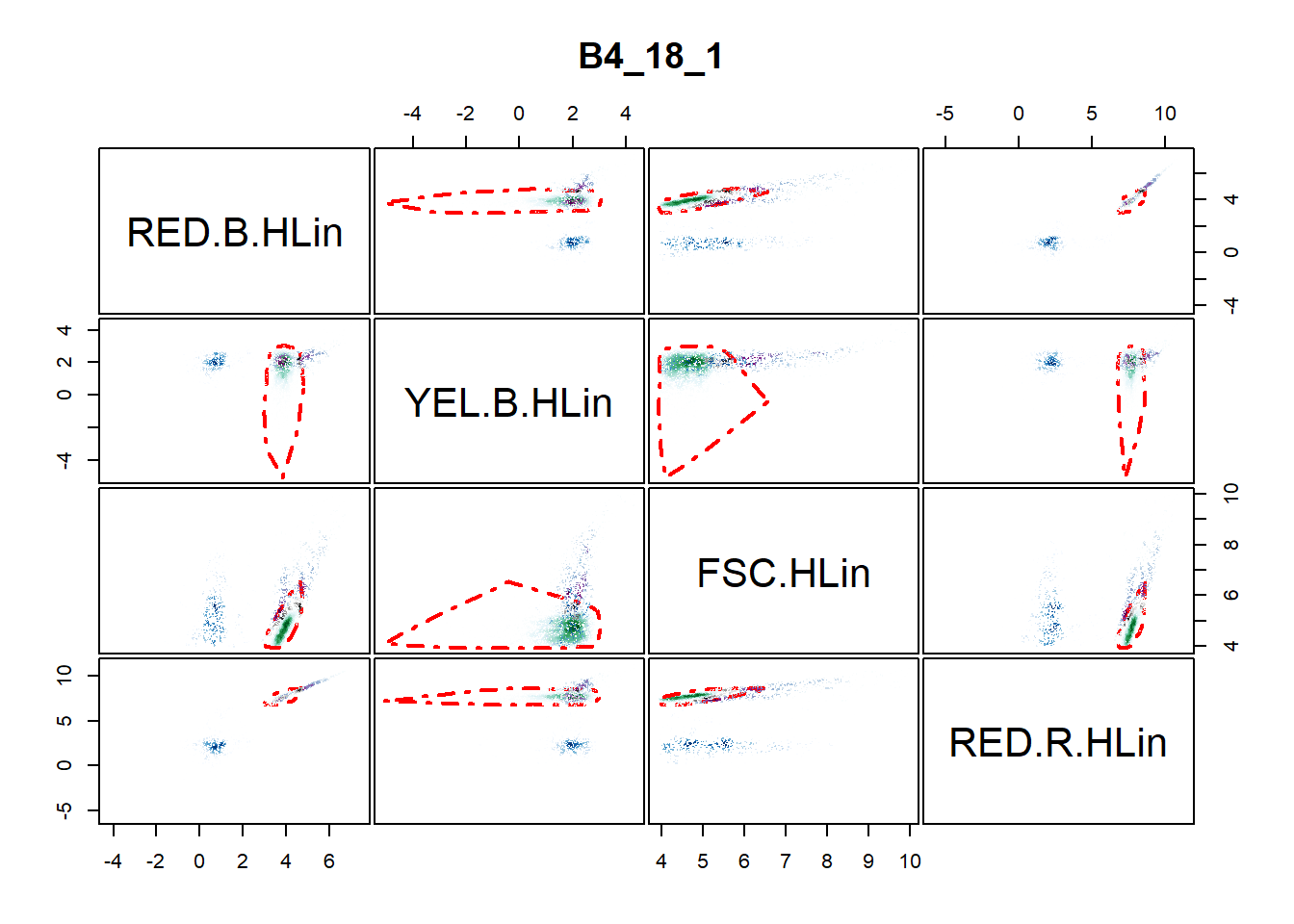

The resulting object is a figure (Figure @ref(fig:emapproach)) and a list containing the following:

1. percentages the final weight for each cluster
2. mus, matrix of means for each channel per cluster
3. sigmas, list containing variance-covariace matrices for each cluster,
4. result, flowfile with an expression matrix containing all the measured particles and the associated probability of each particle belonging to a cluster.

Users can examine the means or cluster weights to determine which cluster is of interest, and then filter out particles belonging to that cluster with a certain minimum probability. For example, we demonstrate an example below by filtering out particles belonging to the cluster with the highest weight by at least 80%.

max_cluster_weight <- which(bs4_gate2$percentages == 
  max(bs4_gate2$percentages))
cluster_name <- paste("Cluster", "Prob", 
  max_cluster_weight, sep = "_")
reduced_frame <- which(bs4_gate2$result[, cluster_name] >= 0.80)

The object reduced_frame is a flowframe containing all particles belonging to the largest cluster with probability of at least 80%. Following the same steps or knowledge of these cells, users can filter out particles belonging to certain clusters with characteristics of interest to them.

Gating Debris and cyanobacteria in biculture

The second file used for demonstration contains both BS4 and BS5 cyanobacteria cells.

flowfile2_path <- system.file("extdata", "B4_B5_18_1.fcs", package = "cyanoFilter",
  mustWork = TRUE)
flowfile2 <- read.FCS(flowfile2_path, alter.names = TRUE,
  transformation = FALSE, emptyValue = FALSE,
  dataset = 1)
flowfile2
> flowFrame object ' BI_18_1'
> with 12665 cells and 11 observables:
>            name                                desc range    minRange
> $P1    FSC.HLin          Forward Scatter (FSC-HLin) 1e+05    0.000000
> $P2    SSC.HLin             Side Scatter (SSC-HLin) 1e+05  -15.474201
> $P3  GRN.B.HLin   Green-B Fluorescence (GRN-B-HLin) 1e+05  -25.141722
> $P4  YEL.B.HLin  Yellow-B Fluorescence (YEL-B-HLin) 1e+05  -13.833652
> $P5  RED.B.HLin     Red-B Fluorescence (RED-B-HLin) 1e+05   -7.098767
> $P6  NIR.B.HLin Near IR-B Fluorescence (NIR-B-HLin) 1e+05   -7.817278
> $P7  RED.R.HLin     Red-R Fluorescence (RED-R-HLin) 1e+05  -32.829483
> $P8  NIR.R.HLin Near IR-R Fluorescence (NIR-R-HLin) 1e+05  -15.511206
> $P9    SSC.ALin        Side Scatter Area (SSC-ALin) 1e+05    0.000000
> $P10      SSC.W          Side Scatter Width (SSC-W) 1e+05 -111.000000
> $P11       TIME                                Time 1e+05    0.000000
>      maxRange
> $P1     99999
> $P2     99999
> $P3     99999
> $P4     99999
> $P5     99999
> $P6     99999
> $P7     99999
> $P8     99999
> $P9     99999
> $P10    99999
> $P11    99999
> 368 keywords are stored in the 'description' slot

All the steps previously demonstrated remains unchanged, s we carry it all out in one huge code chunk.

flowfile_nona2 <- nona(x = flowfile2)
pair_plot(flowfile_nona2, notToPlot = "TIME")

#natural logarithm transformation
flowfile_noneg2 <- noneg(x = flowfile_nona2)
flowfile_logtrans2 <- lnTrans(x = flowfile_noneg2, 
  notToTransform = c("SSC.W", "TIME"))
pair_plot(flowfile_logtrans2, notToPlot = "TIME")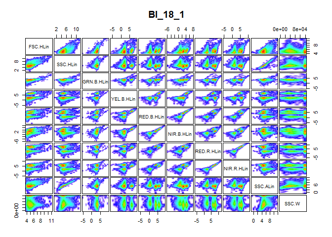

#gating margin events
flowfile_marginout2 <- cellmargin(flow.frame = flowfile_logtrans2,
  Channel = 'SSC.W', type = 'estimate', y_toplot = "FSC.HLin")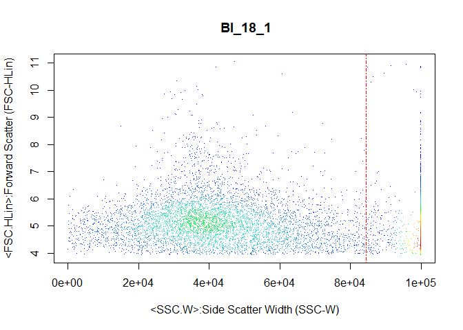

Again we use the two channels measuring cholorophyll a and phycoerythrin, but we set the interest option to both-right. This means that we are expecting the cyanobacteria cells to be on the right of channel 1.

bs45_gate1 <- celldebris_nc(flowfile_marginout2$reducedflowframe, 
  channel1 = "RED.B.HLin", channel2 = "YEL.B.HLin", 
  interest = "both-right", to_retain = "refined" )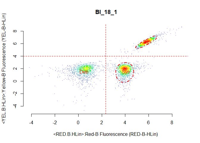

For the EM clustering approach, nothing changes as well. However, users must analyse the result of the clustering to determine which cluster is of interest.

bs4_gate2 <- celldebris_emclustering(flowfile_marginout$reducedflowframe, 
  channels =  c("RED.B.HLin", "YEL.B.HLin", "FSC.HLin", "RED.R.HLin"), 
  ncluster = 4, min.itera = 20, classifier = 0.8)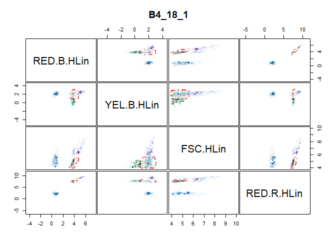

License

This is a free to use package for anyone who has the need.