Cross-Validation for Model Selection
Authors: Ludvig R. Olsen ( r-pkgs@ludvigolsen.dk ), Hugh Benjamin Zachariae
License: MIT
Started: October 2016
![]()
![]()

![]()
R package for model evaluation and comparison.
Currently supports regression ('gaussian'), binary classification ('binomial'), and (some functions only) multiclass classification ('multinomial'). Many of the functions allow parallelization, e.g. through the doParallel package.
| Function | Description |
|---|---|
cross_validate() |
Cross-validate linear models with lm()/lmer()/glm()/glmer() |
cross_validate_fn() |
Cross-validate a custom model function |
validate() |
Validate linear models with (lm/lmer/glm/glmer) |
validate_fn() |
Validate a custom model function |
evaluate() |
Evaluate predictions with a large set of metrics |
baseline()baseline_gaussian()baseline_binomial()baseline_multinomial() |
Perform baseline evaluations of a dataset |
| Function | Description |
|---|---|
confusion_matrix() |
Create a confusion matrix from predictions and targets |
evaluate_residuals() |
Evaluate residuals from a regression task |
most_challenging() |
Find the observations that were the most challenging to predict |
summarize_metrics() |
Summarize numeric columns with a set of descriptors |
| Function | Description |
|---|---|
combine_predictors() |
Generate model formulas from a list of predictors |
reconstruct_formulas() |
Extract formulas from output tibble |
simplify_formula() |
Remove inline functions with more from a formula object |
| Function | Description |
|---|---|
plot_confusion_matrix() |
Plot a confusion matrix |
plot_metric_density() |
Create a density plot for a metric column |
font() |
Set font settings for plotting functions (currently only plot_confusion_matrix()) |
| Function | Description |
|---|---|
model_functions() |
Example model functions for cross_validate_fn() |
predict_functions() |
Example predict functions for cross_validate_fn() |
preprocess_functions() |
Example preprocess functions for cross_validate_fn() |
update_hyperparameters() |
Manage hyperparameters in custom model functions |
| Function | Description |
|---|---|
select_metrics() |
Select the metric columns from the output |
select_definitions() |
Select the model-defining columns from the output |
gaussian_metrics()binomial_metrics()multinomial_metrics() |
Create list of metrics for the common metrics argument |
multiclass_probability_tibble() |
Generate a multiclass probability tibble |
| Name | Description |
|---|---|
participant.scores |
Made-up experiment data with 10 participants and two diagnoses |
wines |
A list of wine varieties in an approximately Zipfian distribution |
musicians |
Made-up data on 60 musicians in 4 groups for multiclass classification |
predicted.musicians |
Predictions by 3 classifiers of the 4 classes in the musicians dataset |
precomputed.formulas |
Fixed effect combinations for model formulas with/without two- and three-way interactions |
compatible.formula.terms |
162,660 pairs of compatible terms for building model formulas with up to 15 fixed effects |
Check
NEWS.mdfor the full list of changes.
Version 1.0.0 contained multiple breaking changes. Please see NEWS.md. (13th of April 2020)
cv_plot() has been removed.
Fixes bug in evaluate(), when used on a grouped data frame. The row order in the output was not guaranteed to fit with the grouping keys. If you have used evaluate() on a grouped data frame, please rerun to make sure your results are correct! (30th of November
In cross_validate() and validate(), the models argument is renamed to formulas and the model_verbose argument is renamed to verbose. Further, the link argument is hard-deprecated and will throw an error if used.
Multinomial AUC is now calculated with pROC::multiclass.roc.
cross_validate_fn() and validate_fn() now take the preprocess_fn, preprocess_once, and hyperparameters arguments. The predict_type argument has been removed.
cross_validate_fn() and validate_fn() are added. (Cross-)validate custom model functions.
CRAN:
install.packages(“cvms”)
Development version:
install.packages(“devtools”)
devtools::install_github(“LudvigOlsen/groupdata2”)
devtools::install_github(“LudvigOlsen/cvms”)
library(cvms)
library(groupdata2)   # fold() partition()
library(knitr)        # kable()
library(dplyr)        # %>% arrange()
library(ggplot2)The dataset participant.scores comes with cvms:
Create a grouping factor for subsetting of folds using groupdata2::fold(). Order the dataset by the folds:
# Set seed for reproducibility
set.seed(7)

# Fold data
data <- fold(
  data = data, k = 4,
  cat_col = 'diagnosis',
  id_col = 'participant') %>%
  arrange(.folds)

# Show first 15 rows of data
data %>% head(15) %>% kable()| participant | age | diagnosis | score | session | .folds |
|---|---|---|---|---|---|
| 9 | 34 | 0 | 33 | 1 | 1 |
| 9 | 34 | 0 | 53 | 2 | 1 |
| 9 | 34 | 0 | 66 | 3 | 1 |
| 8 | 21 | 1 | 16 | 1 | 1 |
| 8 | 21 | 1 | 32 | 2 | 1 |
| 8 | 21 | 1 | 44 | 3 | 1 |
| 2 | 23 | 0 | 24 | 1 | 2 |
| 2 | 23 | 0 | 40 | 2 | 2 |
| 2 | 23 | 0 | 67 | 3 | 2 |
| 1 | 20 | 1 | 10 | 1 | 2 |
| 1 | 20 | 1 | 24 | 2 | 2 |
| 1 | 20 | 1 | 45 | 3 | 2 |
| 6 | 31 | 1 | 14 | 1 | 2 |
| 6 | 31 | 1 | 25 | 2 | 2 |
| 6 | 31 | 1 | 30 | 3 | 2 |
CV1 <- cross_validate(
  data = data,
  formulas = "score ~ diagnosis",
  fold_cols = '.folds',
  family = 'gaussian',
  REML = FALSE
)

# Show results
CV1
#> # A tibble: 1 x 21
#>   Fixed  RMSE   MAE `NRMSE(IQR)`  RRSE   RAE RMSLE   AIC  AICc   BIC Predictions
#>   <chr> <dbl> <dbl>        <dbl> <dbl> <dbl> <dbl> <dbl> <dbl> <dbl> <list>
#> 1 diag…  16.4  13.8        0.937 0.900 0.932 0.474  195.  196.  198. <tibble [3…
#> # … with 10 more variables: Results <list>, Coefficients <list>, Folds <int>,
#> #   `Fold Columns` <int>, `Convergence Warnings` <int>, `Singular Fit
#> #   Messages` <int>, `Other Warnings` <int>, `Warnings and Messages` <list>,
#> #   Family <chr>, Dependent <chr>

# Let's take a closer look at the different parts of the output

# Metrics and formulas
CV1 %>% select_metrics() %>% kable()| Fixed | RMSE | MAE | NRMSE(IQR) | RRSE | RAE | RMSLE | AIC | AICc | BIC | Dependent |
|---|---|---|---|---|---|---|---|---|---|---|
| diagnosis | 16.35261 | 13.75772 | 0.9373575 | 0.9004745 | 0.932284 | 0.4736577 | 194.6218 | 195.9276 | 197.9556 | score |
| Dependent | Fixed |
|---|---|
| score | diagnosis |
# Nested predictions
# Note that [[1]] picks predictions for the first row
CV1$Predictions[[1]] %>% head() %>% kable()| Fold Column | Fold | Observation | Target | Prediction |
|---|---|---|---|---|
| .folds | 1 | 1 | 33 | 51.00000 |
| .folds | 1 | 2 | 53 | 51.00000 |
| .folds | 1 | 3 | 66 | 51.00000 |
| .folds | 1 | 4 | 16 | 30.66667 |
| .folds | 1 | 5 | 32 | 30.66667 |
| .folds | 1 | 6 | 44 | 30.66667 |
| Fold Column | Fold | RMSE | MAE | NRMSE(IQR) | RRSE | RAE | RMSLE | AIC | AICc | BIC |
|---|---|---|---|---|---|---|---|---|---|---|
| .folds | 1 | 12.56760 | 10.72222 | 0.6793295 | 0.7825928 | 0.7845528 | 0.3555080 | 209.9622 | 211.1622 | 213.4963 |
| .folds | 2 | 16.60767 | 14.77778 | 1.0379796 | 1.0090512 | 1.1271186 | 0.5805901 | 182.8739 | 184.2857 | 186.0075 |
| .folds | 3 | 15.97355 | 12.87037 | 1.2528275 | 0.7954799 | 0.8644279 | 0.4767100 | 207.9074 | 209.1074 | 211.4416 |
| .folds | 4 | 20.26162 | 16.66049 | 0.7792933 | 1.0147739 | 0.9530367 | 0.4818228 | 177.7436 | 179.1554 | 180.8772 |
# Nested model coefficients
# Note that you have the full p-values,
# but kable() only shows a certain number of digits
CV1$Coefficients[[1]] %>% kable()| Fold Column | Fold | term | estimate | std.error | statistic | p.value |
|---|---|---|---|---|---|---|
| .folds | 1 | (Intercept) | 51.00000 | 5.901264 | 8.642216 | 0.0000000 |
| .folds | 1 | diagnosis | -20.33333 | 7.464574 | -2.723978 | 0.0123925 |
| .folds | 2 | (Intercept) | 53.33333 | 5.718886 | 9.325826 | 0.0000000 |
| .folds | 2 | diagnosis | -19.66667 | 7.565375 | -2.599563 | 0.0176016 |
| .folds | 3 | (Intercept) | 49.77778 | 5.653977 | 8.804030 | 0.0000000 |
| .folds | 3 | diagnosis | -18.77778 | 7.151778 | -2.625610 | 0.0154426 |
| .folds | 4 | (Intercept) | 49.55556 | 5.061304 | 9.791065 | 0.0000000 |
| .folds | 4 | diagnosis | -22.30556 | 6.695476 | -3.331437 | 0.0035077 |
# Additional information about the model
# and the training process
CV1 %>% select(14:21) %>% kable()| Folds | Fold Columns | Convergence Warnings | Singular Fit Messages | Other Warnings | Warnings and Messages | Family | Dependent |
|---|---|---|---|---|---|---|---|
| 4 | 1 | 0 | 0 | 0 | list(Fold Column = character(0), Fold = integer(0), Function = character(0), Type = character(0), Message = character(0)) |
gaussian | score |
CV2 <- cross_validate(
  data = data,
  formulas = "diagnosis~score",
  fold_cols = '.folds',
  family = 'binomial'
)

# Show results
CV2
#> # A tibble: 1 x 29
#>   Fixed `Balanced Accur…    F1 Sensitivity Specificity `Pos Pred Value`
#>   <chr>            <dbl> <dbl>       <dbl>       <dbl>            <dbl>
#> 1 score            0.736 0.821       0.889       0.583            0.762
#> # … with 23 more variables: `Neg Pred Value` <dbl>, AUC <dbl>, `Lower
#> #   CI` <dbl>, `Upper CI` <dbl>, Kappa <dbl>, MCC <dbl>, `Detection
#> #   Rate` <dbl>, `Detection Prevalence` <dbl>, Prevalence <dbl>,
#> #   Predictions <list>, ROC <list>, `Confusion Matrix` <list>, Results <list>,
#> #   Coefficients <list>, Folds <int>, `Fold Columns` <int>, `Convergence
#> #   Warnings` <int>, `Singular Fit Messages` <int>, `Other Warnings` <int>,
#> #   `Warnings and Messages` <list>, `Positive Class` <chr>, Family <chr>,
#> #   Dependent <chr>

# Let's take a closer look at the different parts of the output
# We won't repeat the parts too similar to those in Gaussian

# Metrics
CV2 %>% select(1:9) %>% kable(digits = 5)| Fixed | Balanced Accuracy | F1 | Sensitivity | Specificity | Pos Pred Value | Neg Pred Value | AUC | Lower CI |
|---|---|---|---|---|---|---|---|---|
| score | 0.73611 | 0.82051 | 0.88889 | 0.58333 | 0.7619 | 0.77778 | 0.76852 | 0.59627 |
| Upper CI | Kappa | MCC | Detection Rate | Detection Prevalence | Prevalence |
|---|---|---|---|---|---|
| 0.9407669 | 0.4927536 | 0.5048268 | 0.5333333 | 0.7 | 0.6 |
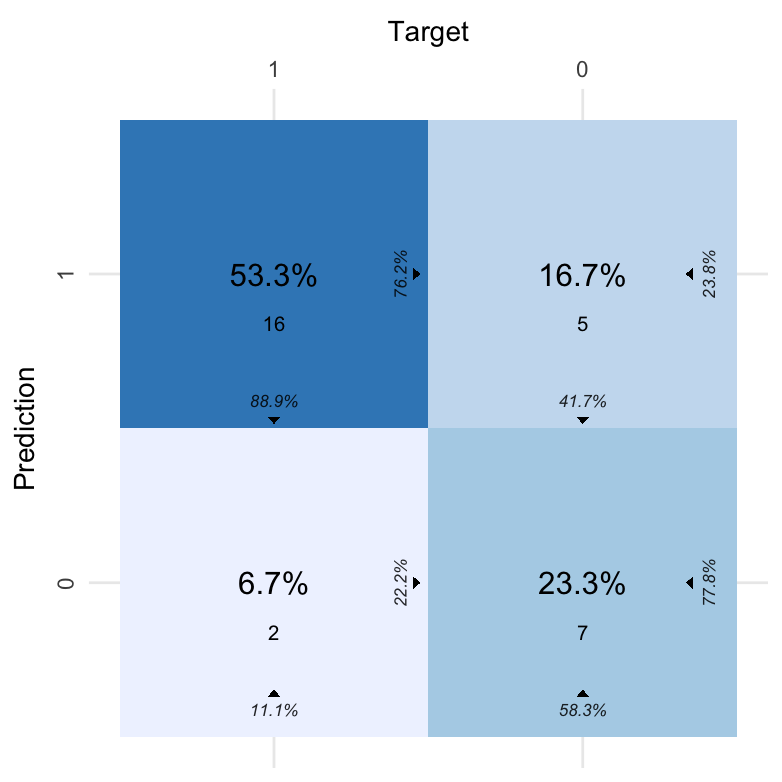
| Fold Column | Prediction | Target | Pos_0 | Pos_1 | N |
|---|---|---|---|---|---|
| .folds | 0 | 0 | TP | TN | 7 |
| .folds | 1 | 0 | FN | FP | 5 |
| .folds | 0 | 1 | FP | FN | 2 |
| .folds | 1 | 1 | TN | TP | 16 |
model_formulas <- c("score ~ diagnosis", "score ~ age")
mixed_model_formulas <- c("score ~ diagnosis + (1|session)",
"score ~ age + (1|session)")CV3 <- cross_validate(
data = data,
formulas = model_formulas,
fold_cols = '.folds',
family = 'gaussian',
REML = FALSE
)
# Show results
CV3
#> # A tibble: 2 x 21
#> Fixed RMSE MAE `NRMSE(IQR)` RRSE RAE RMSLE AIC AICc BIC Predictions
#> <chr> <dbl> <dbl> <dbl> <dbl> <dbl> <dbl> <dbl> <dbl> <dbl> <list>
#> 1 diag… 16.4 13.8 0.937 0.900 0.932 0.474 195. 196. 198. <tibble [3…
#> 2 age 22.4 18.9 1.35 1.23 1.29 0.618 201. 202. 204. <tibble [3…
#> # … with 10 more variables: Results <list>, Coefficients <list>, Folds <int>,
#> # `Fold Columns` <int>, `Convergence Warnings` <int>, `Singular Fit
#> # Messages` <int>, `Other Warnings` <int>, `Warnings and Messages` <list>,
#> # Family <chr>, Dependent <chr>CV4 <- cross_validate(
data = data,
formulas = mixed_model_formulas,
fold_cols = '.folds',
family = 'gaussian',
REML = FALSE
)
# Show results
CV4
#> # A tibble: 2 x 22
#> Fixed RMSE MAE `NRMSE(IQR)` RRSE RAE RMSLE AIC AICc BIC Predictions
#> <chr> <dbl> <dbl> <dbl> <dbl> <dbl> <dbl> <dbl> <dbl> <dbl> <list>
#> 1 diag… 7.95 6.41 0.438 0.432 0.428 0.226 176. 178. 180. <tibble [3…
#> 2 age 17.5 16.2 1.08 0.953 1.11 0.480 194. 196. 198. <tibble [3…
#> # … with 11 more variables: Results <list>, Coefficients <list>, Folds <int>,
#> # `Fold Columns` <int>, `Convergence Warnings` <int>, `Singular Fit
#> # Messages` <int>, `Other Warnings` <int>, `Warnings and Messages` <list>,
#> # Family <chr>, Dependent <chr>, Random <chr>Instead of only dividing our data into folds once, we can do it multiple times and average the results. As the models can be ranked differently with different splits, this is generally preferable.
Let’s first add some extra fold columns. We will use the num_fold_cols argument to add 3 unique fold columns. We tell fold() to keep the existing fold column and simply add three extra columns. We could also choose to remove the existing fold column, if, for instance, we were changing the number of folds (k). Note, that the original fold column will be renamed to ".folds_1".
# Set seed for reproducibility
set.seed(2)

# Fold data
data <- fold(
  data = data, k = 4,
  cat_col = 'diagnosis',
  id_col = 'participant',
  num_fold_cols = 3,
  handle_existing_fold_cols = "keep"
)

# Show first 15 rows of data
data %>% head(10) %>% kable()| participant | age | diagnosis | score | session | .folds_1 | .folds_2 | .folds_3 | .folds_4 |
|---|---|---|---|---|---|---|---|---|
| 10 | 32 | 0 | 29 | 1 | 4 | 4 | 3 | 1 |
| 10 | 32 | 0 | 55 | 2 | 4 | 4 | 3 | 1 |
| 10 | 32 | 0 | 81 | 3 | 4 | 4 | 3 | 1 |
| 2 | 23 | 0 | 24 | 1 | 2 | 3 | 1 | 2 |
| 2 | 23 | 0 | 40 | 2 | 2 | 3 | 1 | 2 |
| 2 | 23 | 0 | 67 | 3 | 2 | 3 | 1 | 2 |
| 4 | 21 | 0 | 35 | 1 | 3 | 2 | 4 | 4 |
| 4 | 21 | 0 | 50 | 2 | 3 | 2 | 4 | 4 |
| 4 | 21 | 0 | 78 | 3 | 3 | 2 | 4 | 4 |
| 9 | 34 | 0 | 33 | 1 | 1 | 1 | 2 | 3 |
Now, let’s cross-validate the four fold columns. We use paste0() to create the four column names:
CV5 <- cross_validate(
  data = data,
  formulas = c("diagnosis ~ score",
               "diagnosis ~ score + age"),
  fold_cols = paste0(".folds_", 1:4),
  family = 'binomial'
)

# Show results
CV5
#> # A tibble: 2 x 29
#>   Fixed `Balanced Accur…    F1 Sensitivity Specificity `Pos Pred Value`
#>   <chr>            <dbl> <dbl>       <dbl>       <dbl>            <dbl>
#> 1 score            0.729 0.813       0.875       0.583            0.759
#> 2 scor…            0.545 0.643       0.653       0.438            0.635
#> # … with 23 more variables: `Neg Pred Value` <dbl>, AUC <dbl>, `Lower
#> #   CI` <dbl>, `Upper CI` <dbl>, Kappa <dbl>, MCC <dbl>, `Detection
#> #   Rate` <dbl>, `Detection Prevalence` <dbl>, Prevalence <dbl>,
#> #   Predictions <list>, ROC <list>, `Confusion Matrix` <list>, Results <list>,
#> #   Coefficients <list>, Folds <int>, `Fold Columns` <int>, `Convergence
#> #   Warnings` <int>, `Singular Fit Messages` <int>, `Other Warnings` <int>,
#> #   `Warnings and Messages` <list>, `Positive Class` <chr>, Family <chr>,
#> #   Dependent <chr>

# Subset of the results per fold for the first model
CV5$Results[[1]] %>% select(1:8) %>% kable()| Fold Column | Balanced Accuracy | F1 | Sensitivity | Specificity | Pos Pred Value | Neg Pred Value | AUC |
|---|---|---|---|---|---|---|---|
| .folds_1 | 0.7361111 | 0.8205128 | 0.8888889 | 0.5833333 | 0.7619048 | 0.7777778 | 0.7685185 |
| .folds_2 | 0.7361111 | 0.8205128 | 0.8888889 | 0.5833333 | 0.7619048 | 0.7777778 | 0.7777778 |
| .folds_3 | 0.7083333 | 0.7894737 | 0.8333333 | 0.5833333 | 0.7500000 | 0.7000000 | 0.7476852 |
| .folds_4 | 0.7361111 | 0.8205128 | 0.8888889 | 0.5833333 | 0.7619048 | 0.7777778 | 0.7662037 |
cross_validate_fn() allows us to cross-validate a custom model function, like a support vector machine or a neural network. It works with regression (gaussian), binary classification (binomial), and multiclass classification (multinomial).
It is required to pass a model function and a predict function. Further, it is possible to pass a preprocessing function and a list of hyperparameter values to test with grid search. You can check the requirements for these functions at ?cross_validate_fn.
Let’s cross-validate a support-vector machine using the svm() function from the e1071 package. First, we will create a model function. You can do anything you want inside it, as long as it takes the arguments train_data, formula, and hyperparameters and returns a fitted model object:
# Create model function
#
# train_data : tibble with the training data
# formula : a formula object
# hyperparameters : a named list of hyparameters

svm_model_fn <- function(train_data, formula, hyperparameters){

  # Note that `formula` must be passed first
  # when calling svm(), otherwise it fails
  e1071::svm(
    formula = formula,
    data = train_data,
    kernel = "linear",
    type = "C-classification",
    probability = TRUE
  )
}
We also need a predict function. This will usually wrap the stats::predict() function. The point is to ensure that the predictions have the correct format. In this case, we want a single column with the probability of the positive class. Note, that you do not need to use the formula, hyperparameters, and train_data arguments within your function. These are there for the few cases, where they are needed.
# Create predict function
#
# test_data : tibble with the test data
# model : fitted model object
# formula : a formula object
# hyperparameters : a named list of hyparameters
# train_data : tibble with the training data

svm_predict_fn <- function(test_data, model, formula, hyperparameters, train_data){

  # Predict the test set with the model
  predictions <- stats::predict(
    object = model,
    newdata = test_data,
    allow.new.levels = TRUE,
    probability = TRUE
  )

  # Extract the probabilities
  # Usually the predict function will just
  # output the probabilities directly
  probabilities <- dplyr::as_tibble(
    attr(predictions, "probabilities")
  )

  # Return second column
  # with probabilities of positive class
  probabilities[[2]]
}
With these functions defined, we can cross-validate the support-vector machine:
# Cross-validate svm_model_fn
CV6 <- cross_validate_fn(
  data = data,
  model_fn = svm_model_fn,
  predict_fn = svm_predict_fn,
  formulas = c("diagnosis ~ score", "diagnosis ~ age"),
  fold_cols = '.folds_1',
  type = 'binomial'
)
#> Will cross-validate 2 models. This requires fitting 8 model instances.

CV6
#> # A tibble: 2 x 28
#>   Fixed `Balanced Accur…    F1 Sensitivity Specificity `Pos Pred Value`
#>   <chr>            <dbl> <dbl>       <dbl>       <dbl>            <dbl>
#> 1 score            0.653 0.780       0.889       0.417            0.696
#> 2 age              0.458 0.615       0.667       0.25             0.571
#> # … with 22 more variables: `Neg Pred Value` <dbl>, AUC <dbl>, `Lower
#> #   CI` <dbl>, `Upper CI` <dbl>, Kappa <dbl>, MCC <dbl>, `Detection
#> #   Rate` <dbl>, `Detection Prevalence` <dbl>, Prevalence <dbl>,
#> #   Predictions <list>, ROC <list>, `Confusion Matrix` <list>, Results <list>,
#> #   Coefficients <list>, Folds <int>, `Fold Columns` <int>, `Convergence
#> #   Warnings` <int>, `Other Warnings` <int>, `Warnings and Messages` <list>,
#> # `Positive Class` <chr>, Family <chr>, Dependent <chr>Let’s try with a naïve Bayes classifier as well. First, we will define the model function:
# Create model function
#
# train_data : tibble with the training data
# formula : a formula object
# hyperparameters : a named list of hyparameters

nb_model_fn <- function(train_data, formula, hyperparameters){
  e1071::naiveBayes(
    formula = formula,
    data = train_data
  )
}
And the predict function:
# Create predict function
#
# test_data : tibble with the test data
# model : fitted model object
# formula : a formula object
# hyperparameters : a named list of hyparameters
# train_data : tibble with the training data

nb_predict_fn <- function(test_data, model, formula, hyperparameters, train_data){
  stats::predict(
    object = model,
    newdata = test_data,
    type = "raw",
    allow.new.levels = TRUE)[, 2]
}
With both functions specified, we are ready to cross-validate our naïve Bayes classifier:
CV7 <- cross_validate_fn(
  data = data,
  model_fn = nb_model_fn,
  predict_fn = nb_predict_fn,
  formulas = c("diagnosis ~ score", "diagnosis ~ age"),
  type = 'binomial',
  fold_cols = '.folds_1'
)
#> Will cross-validate 2 models. This requires fitting 8 model instances.

CV7
#> # A tibble: 2 x 28
#>   Fixed `Balanced Accur…    F1 Sensitivity Specificity `Pos Pred Value`
#>   <chr>            <dbl> <dbl>       <dbl>       <dbl>            <dbl>
#> 1 score            0.736 0.821       0.889       0.583            0.762
#> 2 age              0.25  0.462       0.5         0                0.429
#> # … with 22 more variables: `Neg Pred Value` <dbl>, AUC <dbl>, `Lower
#> #   CI` <dbl>, `Upper CI` <dbl>, Kappa <dbl>, MCC <dbl>, `Detection
#> #   Rate` <dbl>, `Detection Prevalence` <dbl>, Prevalence <dbl>,
#> #   Predictions <list>, ROC <list>, `Confusion Matrix` <list>, Results <list>,
#> #   Coefficients <list>, Folds <int>, `Fold Columns` <int>, `Convergence
#> #   Warnings` <int>, `Other Warnings` <int>, `Warnings and Messages` <list>,
#> # `Positive Class` <chr>, Family <chr>, Dependent <chr>If we wish to investigate why some observations are harder to predict than others, we should start by identifying the most challenging observations. This can be done with most_challenging().
Let’s first extract the predictions from some of the cross-validation results:
glm_predictions <- dplyr::bind_rows(CV5$Predictions, .id = "Model")
svm_predictions <- dplyr::bind_rows(CV6$Predictions, .id = "Model")
nb_predictions <- dplyr::bind_rows(CV7$Predictions, .id = "Model")
predictions <- dplyr::bind_rows(
  glm_predictions,
  svm_predictions,
  nb_predictions,
  .id = "Architecture"
)
predictions[["Target"]] <- as.character(predictions[["Target"]])

predictions
#> # A tibble: 360 x 8
#>    Architecture Model `Fold Column`  Fold Observation Target Prediction
#>    <chr>        <chr> <chr>         <int>       <int> <chr>       <dbl>
#>  1 1            1     .folds_1          1          10 0           0.721
#>  2 1            1     .folds_1          1          11 0           0.422
#>  3 1            1     .folds_1          1          12 0           0.242
#>  4 1            1     .folds_1          1          28 1           0.884
#>  5 1            1     .folds_1          1          29 1           0.734
#>  6 1            1     .folds_1          1          30 1           0.563
#>  7 1            1     .folds_1          2           4 0           0.831
#>  8 1            1     .folds_1          2           5 0           0.620
#>  9 1            1     .folds_1          2           6 0           0.202
#> 10 1            1     .folds_1          2          13 1           0.928
#> # … with 350 more rows, and 1 more variable: `Predicted Class` <chr>
Now, let’s find the overall most difficult to predict observations. most_challenging() calculates the Accuracy, MAE, and Cross-Entropy for each prediction. We can then extract the observations with the ~20% highest MAE scores. Note that most_challenging() works with grouped data frames as well.
challenging <- most_challenging(
  data = predictions,
  prediction_cols = "Prediction",
  type = "binomial",
  threshold = 0.20,
  threshold_is = "percentage"
)

challenging
#> # A tibble: 6 x 7
#>   Observation Correct Incorrect Accuracy   MAE `Cross Entropy`  `<=`
#>         <int>   <int>     <int>    <dbl> <dbl>           <dbl> <dbl>
#> 1          21       1        11   0.0833 0.820            2.10 0.615
#> 2           4       0        12   0      0.783            1.66 0.615
#> 3          10       0        12   0      0.774            1.57 0.615
#> 4          20       1        11   0.0833 0.742            1.50 0.615
#> 5           1       1        11   0.0833 0.733            1.39 0.615
#> 6           7       0        12   0      0.690            1.22 0.615
We can then extract the difficult observations from the dataset. First, we add an index to the dataset. Then, we perform a right-join, to only get the rows that are in the challenging data frame.
# Index with values 1:30
data[["Observation"]] <- seq_len(nrow(data))

# Add information to the challenging observations
challenging <- data %>%
  # Remove fold columns for clarity
  dplyr::select(-c(.folds_1, .folds_2, .folds_3, .folds_4)) %>%
  # Add the scores
  dplyr::right_join(challenging, by = "Observation")

challenging %>% kable()| participant | age | diagnosis | score | session | Observation | Correct | Incorrect | Accuracy | MAE | Cross Entropy | <= |
|---|---|---|---|---|---|---|---|---|---|---|---|
| 5 | 32 | 1 | 62 | 3 | 21 | 1 | 11 | 0.0833333 | 0.8199538 | 2.097782 | 0.6145233 |
| 2 | 23 | 0 | 24 | 1 | 4 | 0 | 12 | 0.0000000 | 0.7832189 | 1.664472 | 0.6145233 |
| 9 | 34 | 0 | 33 | 1 | 10 | 0 | 12 | 0.0000000 | 0.7735253 | 1.568240 | 0.6145233 |
| 5 | 32 | 1 | 54 | 2 | 20 | 1 | 11 | 0.0833333 | 0.7419556 | 1.497591 | 0.6145233 |
| 10 | 32 | 0 | 29 | 1 | 1 | 1 | 11 | 0.0833333 | 0.7333863 | 1.390259 | 0.6145233 |
| 4 | 21 | 0 | 35 | 1 | 7 | 0 | 12 | 0.0000000 | 0.6896729 | 1.218275 | 0.6145233 |
Note: You may have to scroll to the right in the table.
We can also evaluate predictions from a model trained outside cvms. This works with regression ('gaussian'), binary classification ('binomial'), and multiclass classification ('multinomial').
Extract the targets and predictions from the first cross-validation we performed and evaluate it with evaluate(). We group the data frame by the Fold column to evaluate each fold separately:
# Extract the predictions from the first cross-validation
predictions <- CV1$Predictions[[1]]
predictions %>% head(6) %>% kable()| Fold Column | Fold | Observation | Target | Prediction |
|---|---|---|---|---|
| .folds | 1 | 1 | 33 | 51.00000 |
| .folds | 1 | 2 | 53 | 51.00000 |
| .folds | 1 | 3 | 66 | 51.00000 |
| .folds | 1 | 4 | 16 | 30.66667 |
| .folds | 1 | 5 | 32 | 30.66667 |
| .folds | 1 | 6 | 44 | 30.66667 |
# Evaluate the predictions per fold
predictions %>%
  group_by(Fold) %>%
  evaluate(
    target_col = "Target",
    prediction_cols = "Prediction",
    type = "gaussian"
  )
#> # A tibble: 4 x 8
#>    Fold  RMSE   MAE `NRMSE(IQR)`  RRSE   RAE RMSLE Predictions
#>   <int> <dbl> <dbl>        <dbl> <dbl> <dbl> <dbl> <list>
#> 1     1  12.6  10.7        0.679 0.783 0.785 0.356 <tibble [6 × 3]>
#> 2     2  16.6  14.8        1.04  1.01  1.13  0.581 <tibble [9 × 3]>
#> 3     3  16.0  12.9        1.25  0.795 0.864 0.477 <tibble [6 × 3]>
#> 4 4 20.3 16.7 0.779 1.01 0.953 0.482 <tibble [9 × 3]>We can do the same for the predictions from the second, binomial cross-validation:
# Extract the predictions from the second cross-validation
predictions <- CV2$Predictions[[1]]
predictions %>% head(6) %>% kable()| Fold Column | Fold | Observation | Target | Prediction | Predicted Class |
|---|---|---|---|---|---|
| .folds | 1 | 1 | 0 | 0.7214054 | 1 |
| .folds | 1 | 2 | 0 | 0.4216125 | 0 |
| .folds | 1 | 3 | 0 | 0.2423024 | 0 |
| .folds | 1 | 4 | 1 | 0.8837986 | 1 |
| .folds | 1 | 5 | 1 | 0.7339631 | 1 |
| .folds | 1 | 6 | 1 | 0.5632255 | 1 |
# Evaluate the predictions per fold
predictions %>%
  group_by(Fold) %>%
  evaluate(
    target_col = "Target",
    prediction_cols = "Prediction",
    type = "binomial"
  )
#> # A tibble: 4 x 19
#>    Fold `Balanced Accur…    F1 Sensitivity Specificity `Pos Pred Value`
#>   <int>            <dbl> <dbl>       <dbl>       <dbl>            <dbl>
#> 1     1            0.833 0.857       1           0.667             0.75
#> 2     2            0.667 0.857       1           0.333             0.75
#> 3     3            0.833 0.857       1           0.667             0.75
#> 4     4            0.667 0.727       0.667       0.667             0.8
#> # … with 13 more variables: `Neg Pred Value` <dbl>, AUC <dbl>, `Lower
#> #   CI` <dbl>, `Upper CI` <dbl>, Kappa <dbl>, MCC <dbl>, `Detection
#> #   Rate` <dbl>, `Detection Prevalence` <dbl>, Prevalence <dbl>,
#> #   Predictions <list>, ROC <list>, `Confusion Matrix` <list>, `Positive
#> # Class` <chr>We will use the multiclass_probability_tibble() helper to generate a data frame with predicted probabilities for three classes, along with the predicted class and the target class. Then, we will 1) evaluate the three probability columns against the targets (preferable format), and 2) evaluate the predicted classes against the targets:
# Create dataset for multinomial evaluation
multiclass_data <- multiclass_probability_tibble(
  num_classes = 3, # Here, number of predictors
  num_observations = 30,
  apply_softmax = TRUE,
  add_predicted_classes = TRUE,
  add_targets = TRUE)

multiclass_data
#> # A tibble: 30 x 5
#>    class_1 class_2 class_3 `Predicted Class` Target
#>      <dbl>   <dbl>   <dbl> <chr>             <chr>
#>  1   0.200   0.490   0.309 class_2           class_2
#>  2   0.256   0.255   0.489 class_3           class_2
#>  3   0.255   0.423   0.322 class_2           class_2
#>  4   0.391   0.316   0.293 class_1           class_2
#>  5   0.314   0.364   0.321 class_2           class_1
#>  6   0.258   0.449   0.293 class_2           class_1
#>  7   0.406   0.173   0.421 class_3           class_3
#>  8   0.317   0.273   0.410 class_3           class_1
#>  9   0.351   0.227   0.422 class_3           class_3
#> 10   0.373   0.395   0.233 class_2           class_2
#> # … with 20 more rows

# Evaluate probabilities
# One prediction column *per class*
ev <- evaluate(
  data = multiclass_data,
  target_col = "Target",
  prediction_cols = paste0("class_", 1:3),
  type = "multinomial"
)

ev
#> # A tibble: 1 x 15
#>   `Overall Accura… `Balanced Accur…    F1 Sensitivity Specificity
#>              <dbl>            <dbl> <dbl>       <dbl>       <dbl>
#> 1            0.533            0.646 0.516       0.530       0.762
#> # … with 10 more variables: `Pos Pred Value` <dbl>, `Neg Pred Value` <dbl>,
#> #   Kappa <dbl>, MCC <dbl>, `Detection Rate` <dbl>, `Detection
#> #   Prevalence` <dbl>, Prevalence <dbl>, Predictions <list>, `Confusion
#> #   Matrix` <list>, `Class Level Results` <list>

# The one-vs-all evaluations
ev$`Class Level Results`[[1]]
#> # A tibble: 3 x 13
#>   Class `Balanced Accur…    F1 Sensitivity Specificity `Pos Pred Value`
#>   <chr>            <dbl> <dbl>       <dbl>       <dbl>            <dbl>
#> 1 clas…            0.659 0.526       0.556       0.762            0.5
#> 2 clas…            0.633 0.593       0.533       0.733            0.667
#> 3 clas…            0.646 0.429       0.5         0.792            0.375
#> # … with 7 more variables: `Neg Pred Value` <dbl>, Kappa <dbl>, `Detection
#> #   Rate` <dbl>, `Detection Prevalence` <dbl>, Prevalence <dbl>, Support <int>,
#> #   `Confusion Matrix` <list>

# Evaluate the predicted classes
# One prediction column with the class names
evaluate(
  data = multiclass_data,
  target_col = "Target",
  prediction_cols = "Predicted Class",
  type = "multinomial"
)
#> # A tibble: 1 x 15
#>   `Overall Accura… `Balanced Accur…    F1 Sensitivity Specificity
#>              <dbl>            <dbl> <dbl>       <dbl>       <dbl>
#> 1            0.533            0.646 0.516       0.530       0.762
#> # … with 10 more variables: `Pos Pred Value` <dbl>, `Neg Pred Value` <dbl>,
#> #   Kappa <dbl>, MCC <dbl>, `Detection Rate` <dbl>, `Detection
#> #   Prevalence` <dbl>, Prevalence <dbl>, Predictions <list>, `Confusion
#> # Matrix` <list>, `Class Level Results` <list>While it’s common to find the chance-level baseline analytically (in classification tasks), it’s often possible to get a better evaluation than that by chance. Hence, it is useful to check the range of our metrics when randomly guessing the probabilities.
Usually, we use baseline() on our test set at the start of our modeling process, so we know what level of performance we should beat.
Note: Where baseline() works with all three families (gaussian, binomial and multinomial), each family also has a wrapper function (e.g. baseline_gaussian()) that is easier to use. We use those here.
Start by partitioning the dataset:
# Set seed for reproducibility
set.seed(1)

# Partition the dataset
partitions <- groupdata2::partition(
  participant.scores,
  p = 0.7,
  cat_col = 'diagnosis',
  id_col = 'participant',
  list_out = TRUE
)

train_set <- partitions[[1]]
test_set <- partitions[[2]]Approach: n random sets of predictions are evaluated against the dependent variable in the test set. We also evaluate a set of all 0s and a set of all 1s.
Create the baseline evaluations:
# Perform binomial baseline evaluation
# Note: It's worth enabling parallelization (see ?baseline examples)
binomial_baseline <- baseline_binomial(
  test_data = test_set,
  dependent_col = "diagnosis",
  n = 100
)

binomial_baseline$summarized_metrics
#> # A tibble: 10 x 15
#>    Measure `Balanced Accur…      F1 Sensitivity Specificity `Pos Pred Value`
#>    <chr>              <dbl>   <dbl>       <dbl>       <dbl>            <dbl>
#>  1 Mean               0.496   0.481       0.475       0.517            0.494
#>  2 Median             0.5     0.5         0.5         0.5              0.5
#>  3 SD                 0.130   0.144       0.178       0.181            0.146
#>  4 IQR                0.167   0.195       0.208       0.333            0.200
#>  5 Max                0.833   0.833       0.833       0.833            0.833
#>  6 Min                0.25    0.182       0           0.167            0
#>  7 NAs                0       1           0           0                0
#>  8 INFs               0       0           0           0                0
#>  9 All_0              0.5   NaN           0           1              NaN
#> 10 All_1              0.5     0.667       1           0                0.5
#> # … with 9 more variables: `Neg Pred Value` <dbl>, AUC <dbl>, `Lower CI` <dbl>,
#> #   `Upper CI` <dbl>, Kappa <dbl>, MCC <dbl>, `Detection Rate` <dbl>,
#> #   `Detection Prevalence` <dbl>, Prevalence <dbl>
On average, we can expect an F1 score of approximately 0.481. The maximum F1 score achieved by randomly guessing was 0.833 though. That’s likely because of the small size of the test set, but it illustrates how such information could be useful in a real-life scenario.
The All_1 row shows us that we can achieve an F1 score of 0.667 by always predicting 1. Some model architectures, like neural networks, have a tendency to always predict the majority class. Such a model is quite useless of course, why it is good to be aware of the performance it could achieve. We could also check the confusion matrix for such a pattern.
binomial_baseline$random_evaluations
#> # A tibble: 100 x 20
#>    `Balanced Accur…    F1 Sensitivity Specificity `Pos Pred Value`
#>               <dbl> <dbl>       <dbl>       <dbl>            <dbl>
#>  1            0.417 0.462       0.5         0.333            0.429
#>  2            0.667 0.6         0.5         0.833            0.75
#>  3            0.5   0.571       0.667       0.333            0.5
#>  4            0.417 0.364       0.333       0.5              0.4
#>  5            0.583 0.545       0.5         0.667            0.6
#>  6            0.583 0.545       0.5         0.667            0.6
#>  7            0.667 0.667       0.667       0.667            0.667
#>  8            0.417 0.364       0.333       0.5              0.4
#>  9            0.333 0.333       0.333       0.333            0.333
#> 10            0.583 0.545       0.5         0.667            0.6
#> # … with 90 more rows, and 15 more variables: `Neg Pred Value` <dbl>,
#> #   AUC <dbl>, `Lower CI` <dbl>, `Upper CI` <dbl>, Kappa <dbl>, MCC <dbl>,
#> #   `Detection Rate` <dbl>, `Detection Prevalence` <dbl>, Prevalence <dbl>,
#> #   Predictions <list>, ROC <list>, `Confusion Matrix` <list>, `Positive
#> #   Class` <chr>, Family <chr>, Dependent <chr>
We can plot the distribution of F1 scores from the random evaluations:
# First, remove the NAs from the F1 column
random_evaluations <- binomial_baseline$random_evaluations
random_evaluations <- random_evaluations[!is.na(random_evaluations$F1),]

# Create density plot for F1
plot_metric_density(baseline = random_evaluations,
                    metric = "F1", xlim = c(0, 1))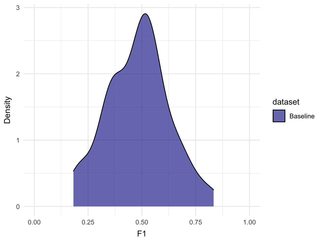
Approach: Creates one-vs-all (binomial) baseline evaluations for n sets of random predictions against the dependent variable, along with sets of all class x,y,z,... predictions.
Create the baseline evaluations:
multiclass_baseline <- baseline_multinomial(
  test_data = multiclass_data,
  dependent_col = "Target",
  n = 100
)

# Summarized metrics
multiclass_baseline$summarized_metrics
#> # A tibble: 15 x 13
#>    Measure `Overall Accura… `Balanced Accur…       F1 Sensitivity Specificity
#>    <chr>              <dbl>            <dbl>    <dbl>       <dbl>       <dbl>
#>  1 Mean              0.330            0.497    0.324       0.329       0.665
#>  2 Median            0.333            0.496    0.325       0.330       0.659
#>  3 SD                0.0823           0.0662   0.0760      0.0904      0.0445
#>  4 IQR               0.108            0.0897   0.0987      0.123       0.0669
#>  5 Max               0.5              0.664    0.499       0.556       0.773
#>  6 Min               0.133            0.352    0.131       0.137       0.562
#>  7 NAs               0                0       10           0           0
#>  8 INFs              0                0        0           0           0
#>  9 CL_Max           NA                0.770    0.688       0.833       0.933
#> 10 CL_Min           NA                0.286    0.0870      0           0.286
#> 11 CL_NAs           NA                0       10           0           0
#> 12 CL_INFs          NA                0        0           0           0
#> 13 All_cl…           0.3              0.5    NaN           0.333       0.667
#> 14 All_cl…           0.5              0.5    NaN           0.333       0.667
#> 15 All_cl…           0.2              0.5    NaN           0.333       0.667
#> # … with 7 more variables: `Pos Pred Value` <dbl>, `Neg Pred Value` <dbl>,
#> #   Kappa <dbl>, MCC <dbl>, `Detection Rate` <dbl>, `Detection
#> #   Prevalence` <dbl>, Prevalence <dbl>
The CL_ measures describe the Class Level Results (aka. one-vs-all evaluations). One of the classes have a maximum Balanced Accuracy score of 0.770, while the maximum Balanced Accuracy in the random evaluations is 0.664.
# Summarized class level results for class 1
multiclass_baseline$summarized_class_level_results %>%
  dplyr::filter(Class == "class_1") %>%
  tidyr::unnest(Results)
#> # A tibble: 10 x 12
#>    Class Measure `Balanced Accur…      F1 Sensitivity Specificity
#>    <chr> <chr>              <dbl>   <dbl>       <dbl>       <dbl>
#>  1 clas… Mean              0.493    0.314       0.339       0.648
#>  2 clas… Median            0.472    0.3         0.333       0.667
#>  3 clas… SD                0.0933   0.119       0.148       0.103
#>  4 clas… IQR               0.127    0.159       0.222       0.143
#>  5 clas… Max               0.770    0.667       0.778       0.905
#>  6 clas… Min               0.286    0.105       0           0.286
#>  7 clas… NAs               0        1           0           0
#>  8 clas… INFs              0        0           0           0
#>  9 clas… All_0             0.5    NaN           0           1
#> 10 clas… All_1             0.5      0.462       1           0
#> # … with 6 more variables: `Pos Pred Value` <dbl>, `Neg Pred Value` <dbl>,
#> #   Kappa <dbl>, `Detection Rate` <dbl>, `Detection Prevalence` <dbl>,
#> #   Prevalence <dbl>

# Random evaluations
# Note, that the class level results for each repetition
# are available as well
multiclass_baseline$random_evaluations
#> # A tibble: 100 x 18
#>    Repetition `Overall Accura… `Balanced Accur…      F1 Sensitivity Specificity
#>         <int>            <dbl>            <dbl>   <dbl>       <dbl>       <dbl>
#>  1          1            0.2              0.401 NaN           0.207       0.594
#>  2          2            0.233            0.427   0.239       0.252       0.602
#>  3          3            0.433            0.564   0.410       0.415       0.712
#>  4          4            0.367            0.529   0.352       0.356       0.702
#>  5          5            0.167            0.394   0.161       0.189       0.600
#>  6          6            0.333            0.496   0.314       0.319       0.673
#>  7          7            0.4              0.534   0.359       0.363       0.705
#>  8          8            0.467            0.608   0.462       0.485       0.731
#>  9          9            0.3              0.476   0.286       0.296       0.655
#> 10         10            0.267            0.430   0.261       0.259       0.602
#> # … with 90 more rows, and 12 more variables: `Pos Pred Value` <dbl>, `Neg Pred
#> #   Value` <dbl>, Kappa <dbl>, MCC <dbl>, `Detection Rate` <dbl>, `Detection
#> #   Prevalence` <dbl>, Prevalence <dbl>, Predictions <list>, `Confusion
#> # Matrix` <list>, `Class Level Results` <list>, Family <chr>, Dependent <chr>Approach: The baseline model (y ~ 1), where 1 is simply the intercept (i.e. mean of y), is fitted on n random subsets of the training set and evaluated on the test set. We also perform an evaluation of the model fitted on the entire training set.
We usually wish to establish whether our predictors add anything useful to our model. We should thus at least do better than a model without any predictors.
Create the baseline evaluations:
gaussian_baseline <- baseline_gaussian(
  test_data = test_set,
  train_data = train_set,
  dependent_col = "score",
  n = 100
)

gaussian_baseline$summarized_metrics
#> # A tibble: 9 x 8
#>   Measure    RMSE      MAE `NRMSE(IQR)`   RRSE      RAE  RMSLE `Training Rows`
#>   <chr>     <dbl>    <dbl>        <dbl>  <dbl>    <dbl>  <dbl>           <dbl>
#> 1 Mean     19.6   15.8           0.944  1.04   1.02     0.559             9.88
#> 2 Median   19.2   15.5           0.925  1.01   1        0.548            10
#> 3 SD        1.19   0.941         0.0575 0.0630 0.0607   0.0303            3.31
#> 4 IQR       0.682  0.00321       0.0328 0.0360 0.000207 0.0189            6
#> 5 Max      26.8   21.8           1.29   1.42   1.41     0.727            15
#> 6 Min      18.9   15.5           0.912  1.00   1        0.541             5
#> 7 NAs       0      0             0      0      0        0                 0
#> 8 INFs      0      0             0      0      0        0                 0
#> 9 All_rows 19.1   15.5           0.923  1.01   1        0.543            18
The All_rows row tells us the performance when fitting the intercept model on the full training set. It is quite close to the mean of the random evaluations.
gaussian_baseline$random_evaluations
#> # A tibble: 100 x 12
#>     RMSE   MAE `NRMSE(IQR)`  RRSE   RAE RMSLE Predictions Coefficients
#>    <dbl> <dbl>        <dbl> <dbl> <dbl> <dbl> <list>      <list>
#>  1  19.1  15.5        0.921  1.01  1    0.544 <tibble [1… <tibble [1 …
#>  2  19.2  15.5        0.926  1.02  1    0.543 <tibble [1… <tibble [1 …
#>  3  19.0  15.5        0.917  1.01  1    0.568 <tibble [1… <tibble [1 …
#>  4  19.0  15.5        0.916  1.00  1    0.566 <tibble [1… <tibble [1 …
#>  5  19.2  15.5        0.927  1.02  1    0.542 <tibble [1… <tibble [1 …
#>  6  19.5  15.5        0.937  1.03  1    0.541 <tibble [1… <tibble [1 …
#>  7  20.4  15.9        0.983  1.08  1.02 0.546 <tibble [1… <tibble [1 …
#>  8  18.9  15.5        0.912  1.00  1    0.558 <tibble [1… <tibble [1 …
#>  9  19.5  15.5        0.939  1.03  1    0.541 <tibble [1… <tibble [1 …
#> 10  18.9  15.5        0.912  1.00  1    0.558 <tibble [1… <tibble [1 …
#> # … with 90 more rows, and 4 more variables: `Training Rows` <int>,
#> #   Family <chr>, Dependent <chr>, Fixed <chr>
Plot the density plot for RMSE:
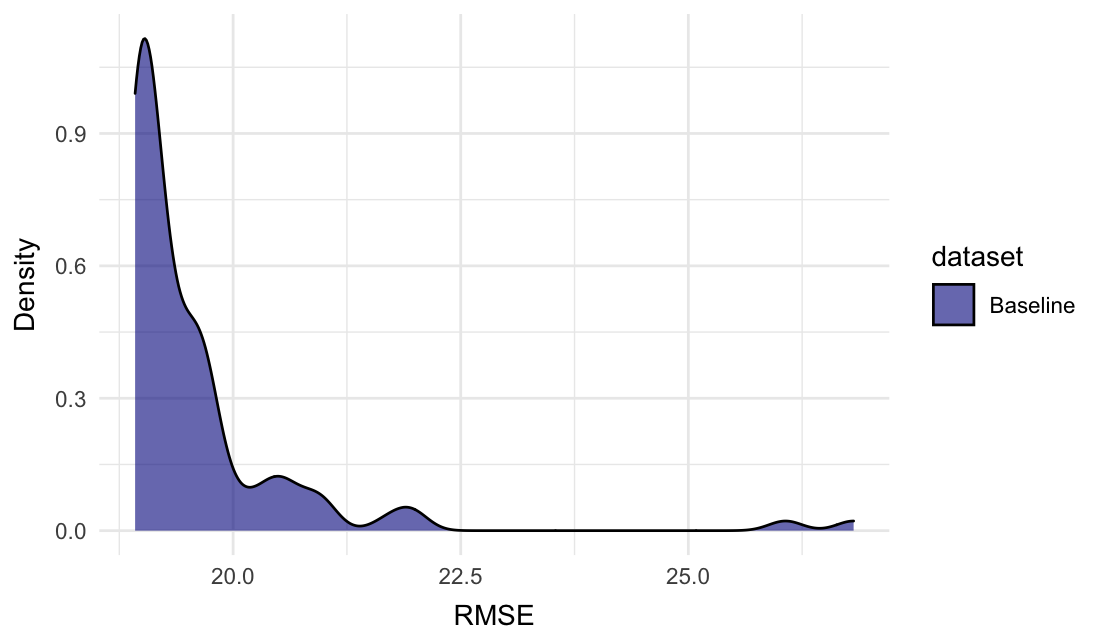
In this instance, the All_rows row might have been enough, as the subsets mainly add higher RMSE scores.
Instead of manually typing all possible model formulas for a set of fixed effects (including the possible interactions), combine_predictors() can do it for you (with some constraints).
When including interactions, >200k formulas have been precomputed for up to 8 fixed effects, with a maximum interaction size of 3, and a maximum of 5 fixed effects per formula. It’s possible to further limit the generated formulas.
We can also append a random effects structure to the generated formulas.
combine_predictors(
  dependent = "y",
  fixed_effects = c("a", "b", "c"),
  random_effects = "(1|d)"
)
#>  [1] "y ~ a + (1|d)"                     "y ~ b + (1|d)"
#>  [3] "y ~ c + (1|d)"                     "y ~ a * b + (1|d)"
#>  [5] "y ~ a * c + (1|d)"                 "y ~ a + b + (1|d)"
#>  [7] "y ~ a + c + (1|d)"                 "y ~ b * c + (1|d)"
#>  [9] "y ~ b + c + (1|d)"                 "y ~ a * b * c + (1|d)"
#> [11] "y ~ a * b + c + (1|d)"             "y ~ a * c + b + (1|d)"
#> [13] "y ~ a + b * c + (1|d)"             "y ~ a + b + c + (1|d)"
#> [15] "y ~ a * b + a * c + (1|d)"         "y ~ a * b + b * c + (1|d)"
#> [17] "y ~ a * c + b * c + (1|d)"         "y ~ a * b + a * c + b * c + (1|d)"
If two or more fixed effects should not be in the same formula, like an effect and its log-transformed version, we can provide them as sublists.