
![]()
![]()
correlation is an easystats package focused on correlation analysis. It’s lightweight, easy to use, and allows for the computation of many different kinds of correlations, such as partial correlations, Bayesian correlations, multilevel correlations, polychoric correlations, biweight, percentage bend or Sheperd’s Pi correlations (types of robust correlation), distance correlation (a type of non-linear correlation) and more, also allowing for combinations between them (for instance, Bayesian partial multilevel correlation).
You can reference the package and its documentation as follows:
Run the following:
![]()
![]()
![]()
Click on the buttons above to access the package documentation and the easystats blog, and check-out these vignettes:
The main function is correlation(), which builds on top of cor_test() and comes with a number of possible options.
cor <- correlation(iris)
cor
## Parameter1   |   Parameter2 |     r |         95% CI |     t |  df |      p |  Method | n_Obs
## ---------------------------------------------------------------------------------------------
## Sepal.Length |  Sepal.Width | -0.12 | [-0.27,  0.04] | -1.44 | 148 | 0.152  | Pearson |   150
## Sepal.Length | Petal.Length |  0.87 | [ 0.83,  0.91] | 21.65 | 148 | < .001 | Pearson |   150
## Sepal.Length |  Petal.Width |  0.82 | [ 0.76,  0.86] | 17.30 | 148 | < .001 | Pearson |   150
## Sepal.Width  | Petal.Length | -0.43 | [-0.55, -0.29] | -5.77 | 148 | < .001 | Pearson |   150
## Sepal.Width  |  Petal.Width | -0.37 | [-0.50, -0.22] | -4.79 | 148 | < .001 | Pearson |   150
## Petal.Length |  Petal.Width |  0.96 | [ 0.95,  0.97] | 43.39 | 148 | < .001 | Pearson |   150
The output is not a square matrix, but a (tidy) dataframe with all correlations tests per row. One can also obtain a matrix using:
summary(cor)
## Parameter    | Petal.Width | Petal.Length | Sepal.Width
## -------------------------------------------------------
## Sepal.Length |     0.82*** |      0.87*** |       -0.12
## Sepal.Width  |    -0.37*** |     -0.43*** |
## Petal.Length |     0.96*** |              |
Note that one can also obtain the full, square and redundant matrix using:
summary(cor, redundant=TRUE)
## Parameter    | Sepal.Length | Sepal.Width | Petal.Length | Petal.Width
## ----------------------------------------------------------------------
## Sepal.Length |      1.00*** |       -0.12 |      0.87*** |     0.82***
## Sepal.Width  |        -0.12 |     1.00*** |     -0.43*** |    -0.37***
## Petal.Length |      0.87*** |    -0.43*** |      1.00*** |     0.96***
## Petal.Width  |      0.82*** |    -0.37*** |      0.96*** |     1.00***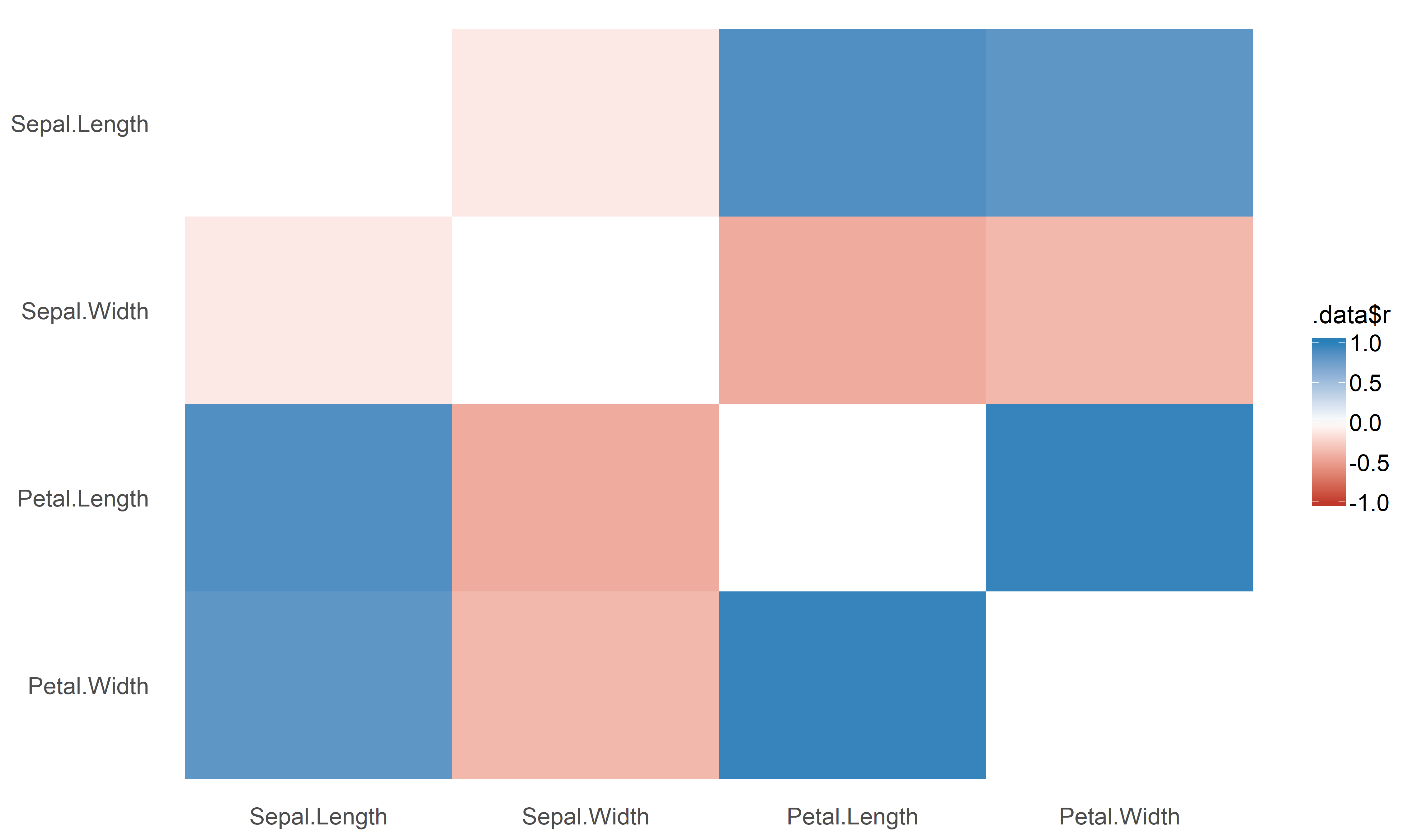
The function also supports stratified correlations, all within the tidyverse workflow!
iris %>%
  select(Species, Sepal.Length, Sepal.Width, Petal.Width) %>%
  group_by(Species) %>%
  correlation()
## Group      |   Parameter1 |  Parameter2 |    r |        95% CI |    t | df |      p |  Method | n_Obs
## -----------------------------------------------------------------------------------------------------
## setosa     | Sepal.Length | Sepal.Width | 0.74 | [ 0.59, 0.85] | 7.68 | 48 | < .001 | Pearson |    50
## setosa     | Sepal.Length | Petal.Width | 0.28 | [ 0.00, 0.52] | 2.01 | 48 | 0.101  | Pearson |    50
## setosa     |  Sepal.Width | Petal.Width | 0.23 | [-0.05, 0.48] | 1.66 | 48 | 0.104  | Pearson |    50
## versicolor | Sepal.Length | Sepal.Width | 0.53 | [ 0.29, 0.70] | 4.28 | 48 | < .001 | Pearson |    50
## versicolor | Sepal.Length | Petal.Width | 0.55 | [ 0.32, 0.72] | 4.52 | 48 | < .001 | Pearson |    50
## versicolor |  Sepal.Width | Petal.Width | 0.66 | [ 0.47, 0.80] | 6.15 | 48 | < .001 | Pearson |    50
## virginica  | Sepal.Length | Sepal.Width | 0.46 | [ 0.20, 0.65] | 3.56 | 48 | 0.002  | Pearson |    50
## virginica  | Sepal.Length | Petal.Width | 0.28 | [ 0.00, 0.52] | 2.03 | 48 | 0.048  | Pearson |    50
## virginica | Sepal.Width | Petal.Width | 0.54 | [ 0.31, 0.71] | 4.42 | 48 | < .001 | Pearson | 50It is very easy to switch to a Bayesian framework.
correlation(iris, bayesian = TRUE)
## Parameter1   |   Parameter2 |   rho |         95% CI |     pd | % in ROPE |    BF |              Prior | n_Obs
## --------------------------------------------------------------------------------------------------------------
## Sepal.Length |  Sepal.Width | -0.11 | [-0.23,  0.02] | 92.10% |    43.90% |  0.51 | Cauchy (0 +- 0.33) |   150
## Sepal.Length | Petal.Length |  0.86 | [ 0.83,  0.90] |   100% |        0% | > 999 | Cauchy (0 +- 0.33) |   150
## Sepal.Length |  Petal.Width |  0.81 | [ 0.76,  0.85] |   100% |        0% | > 999 | Cauchy (0 +- 0.33) |   150
## Sepal.Width  | Petal.Length | -0.41 | [-0.51, -0.30] |   100% |        0% | > 999 | Cauchy (0 +- 0.33) |   150
## Sepal.Width  |  Petal.Width | -0.35 | [-0.46, -0.24] |   100% |     0.02% | > 999 | Cauchy (0 +- 0.33) |   150
## Petal.Length | Petal.Width | 0.96 | [ 0.95, 0.97] | 100% | 0% | > 999 | Cauchy (0 +- 0.33) | 150The correlation package also supports different types of methods, which can deal with correlations between factors!
correlation(iris, include_factors = TRUE, method = "auto")
## Parameter1         |         Parameter2 |     r |         95% CI |      t |  df |      p |         Method | n_Obs
## -----------------------------------------------------------------------------------------------------------------
## Sepal.Length       |        Sepal.Width | -0.12 | [-0.27,  0.04] |  -1.44 | 148 | 0.452  |        Pearson |   150
## Sepal.Length       |       Petal.Length |  0.87 | [ 0.83,  0.91] |  21.65 | 148 | < .001 |        Pearson |   150
## Sepal.Length       |        Petal.Width |  0.82 | [ 0.76,  0.86] |  17.30 | 148 | < .001 |        Pearson |   150
## Sepal.Length       |     Species.setosa | -0.72 | [-0.79, -0.63] | -12.53 | 148 | < .001 | Point-biserial |   150
## Sepal.Length       | Species.versicolor |  0.08 | [-0.08,  0.24] |   0.97 | 148 | 0.452  | Point-biserial |   150
## Sepal.Length       |  Species.virginica |  0.64 | [ 0.53,  0.72] |  10.08 | 148 | < .001 | Point-biserial |   150
## Sepal.Width        |       Petal.Length | -0.43 | [-0.55, -0.29] |  -5.77 | 148 | < .001 |        Pearson |   150
## Sepal.Width        |        Petal.Width | -0.37 | [-0.50, -0.22] |  -4.79 | 148 | < .001 |        Pearson |   150
## Sepal.Width        |     Species.setosa |  0.60 | [ 0.49,  0.70] |   9.20 | 148 | < .001 | Point-biserial |   150
## Sepal.Width        | Species.versicolor | -0.47 | [-0.58, -0.33] |  -6.44 | 148 | < .001 | Point-biserial |   150
## Sepal.Width        |  Species.virginica | -0.14 | [-0.29,  0.03] |  -1.67 | 148 | 0.392  | Point-biserial |   150
## Petal.Length       |        Petal.Width |  0.96 | [ 0.95,  0.97] |  43.39 | 148 | < .001 |        Pearson |   150
## Petal.Length       |     Species.setosa | -0.92 | [-0.94, -0.89] | -29.13 | 148 | < .001 | Point-biserial |   150
## Petal.Length       | Species.versicolor |  0.20 | [ 0.04,  0.35] |   2.51 | 148 | 0.066  | Point-biserial |   150
## Petal.Length       |  Species.virginica |  0.72 | [ 0.63,  0.79] |  12.66 | 148 | < .001 | Point-biserial |   150
## Petal.Width        |     Species.setosa | -0.89 | [-0.92, -0.85] | -23.41 | 148 | < .001 | Point-biserial |   150
## Petal.Width        | Species.versicolor |  0.12 | [-0.04,  0.27] |   1.44 | 148 | 0.452  | Point-biserial |   150
## Petal.Width        |  Species.virginica |  0.77 | [ 0.69,  0.83] |  14.66 | 148 | < .001 | Point-biserial |   150
## Species.setosa     | Species.versicolor | -0.88 | [-0.91, -0.84] | -22.35 | 148 | < .001 |    Tetrachoric |   150
## Species.setosa     |  Species.virginica | -0.88 | [-0.91, -0.84] | -22.35 | 148 | < .001 |    Tetrachoric |   150
## Species.versicolor | Species.virginica | -0.88 | [-0.91, -0.84] | -22.35 | 148 | < .001 | Tetrachoric | 150It also supports partial correlations (as well as Bayesian partial correlations).
iris %>%
  correlation(partial = TRUE) %>%
  summary()
## Parameter    | Petal.Width | Petal.Length | Sepal.Width
## -------------------------------------------------------
## Sepal.Length |    -0.34*** |      0.72*** |     0.63***
## Sepal.Width  |     0.35*** |     -0.62*** |
## Petal.Length | 0.87*** | |Such partial correlations can also be represented as Gaussian graphical models, an increasingly popular tool in psychology:
library(see) # for plotting
library(ggraph) # needs to be loaded

mtcars %>%
  correlation(partial = TRUE) %>%
  plot()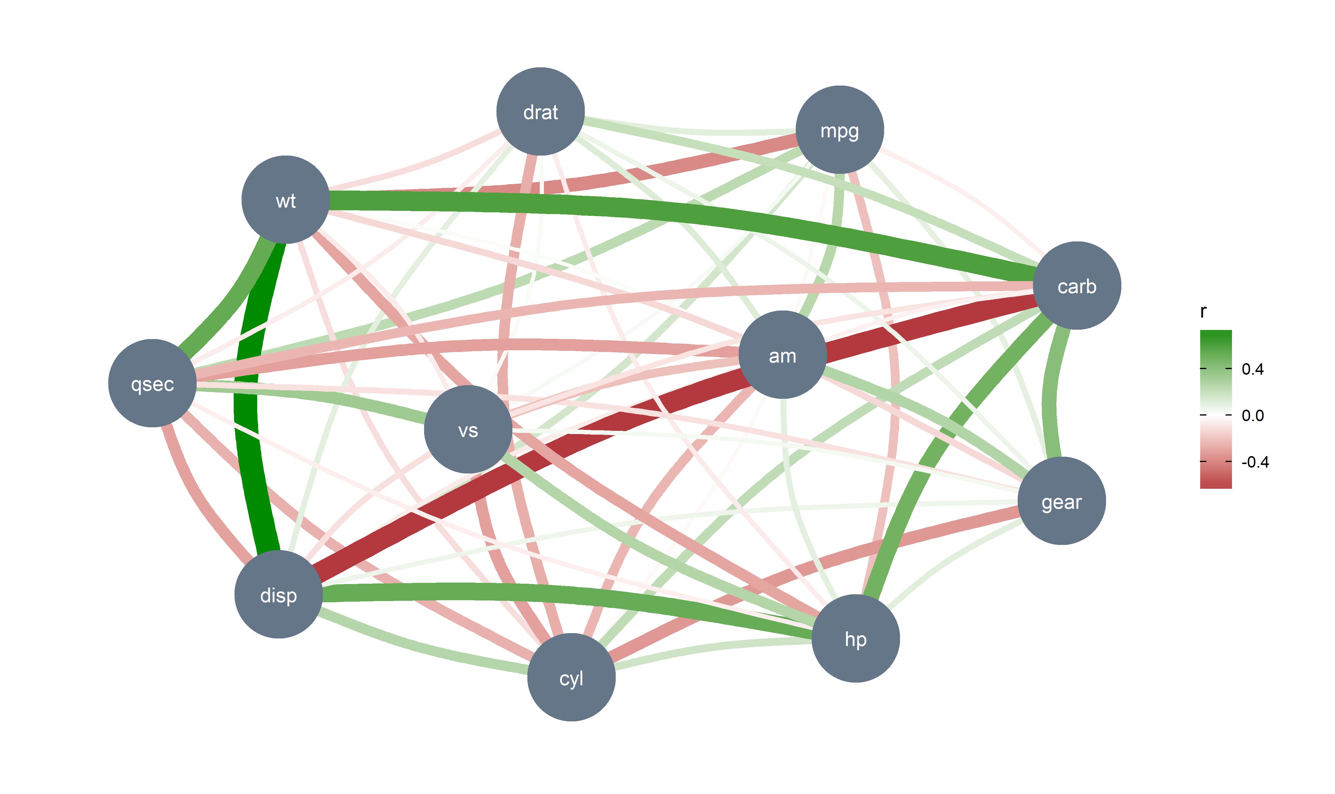
It also provide some cutting-edge methods, such as Multilevel (partial) correlations. These are are partial correlations based on linear mixed models that include the factors as random effects. They can be see as correlations adjusted for some group (hierarchical) variability.
iris %>%
  correlation(partial = TRUE, multilevel = TRUE) %>%
  summary()
## Parameter    | Petal.Width | Petal.Length | Sepal.Width
## -------------------------------------------------------
## Sepal.Length |      -0.17* |      0.71*** |     0.43***
## Sepal.Width  |     0.39*** |       -0.18* |
## Petal.Length |     0.38*** |              |
However, if the partial argument is set to FALSE, it will try to convert the partial coefficient into regular ones.These can be converted back to full correlations: