
![]()
![]()
![]()

The coronavirus package provides a tidy format dataset of the 2019 Novel Coronavirus COVID-19 (2019-nCoV) epidemic. The raw data pulled from the Johns Hopkins University Center for Systems Science and Engineering (JHU CCSE) Coronavirus repository.
More details available here, and a csv format of the package dataset available here
A summary dashboard is available here
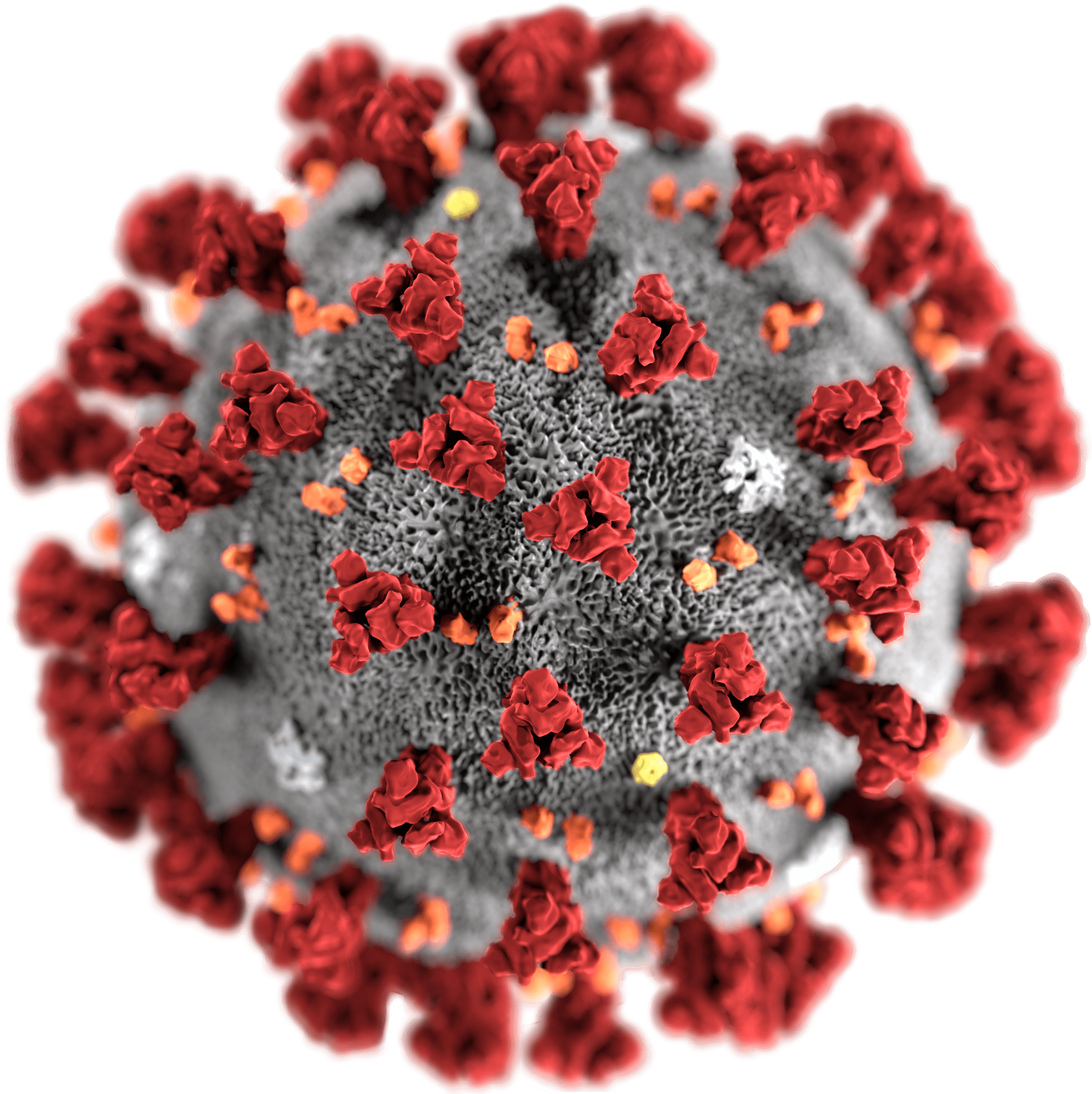
Source: Centers for Disease Control and Prevention’s Public Health Image Library
As this an ongoing situation, frequent changes in the data format may occur, please visit the package news to get updates about those changes
Install the CRAN version:
Install the Github version (refreshed on a daily bases):
While the coronavirus CRAN version is updated every month or two, the Github (Dev) version is updated on a daily bases. The update_dataset function enables to overcome this gap and keep the installed version with the most recent data available on the Github version:
Note: must restart the R session to have the updates available
Alternatively, you can pull the data using the Covid19R project data standard format with the refresh_coronavirus_jhu function:
covid19_df <- refresh_coronavirus_jhu()

head(covid19_df)
#>         date    location location_type location_code location_code_type  data_type value      lat      long
#> 1 2020-05-30 Afghanistan       country            AF         iso_3166_2 deaths_new     3 33.93911 67.709953
#> 2 2020-05-27 Afghanistan       country            AF         iso_3166_2 deaths_new     7 33.93911 67.709953
#> 3 2020-05-29 Afghanistan       country            AF         iso_3166_2 deaths_new    11 33.93911 67.709953
#> 4 2020-02-01 Afghanistan       country            AF         iso_3166_2  cases_new     0 33.93911 67.709953
#> 5 2020-05-26 Afghanistan       country            AF         iso_3166_2 deaths_new     1 33.93911 67.709953
#> 6 2020-06-01 Afghanistan country AF iso_3166_2 deaths_new 8 33.93911 67.709953This coronavirus dataset has the following fields:
date - The date of the summaryprovince - The province or state, when applicablecountry - The country or region namelat - Latitude pointlong - Longitude pointtype - the type of case (i.e., confirmed, death)cases - the number of daily cases (corresponding to the case type)head(coronavirus)
#> date province country lat long type cases
#> 1 2020-01-22 Afghanistan 33.93911 67.709953 confirmed 0
#> 2 2020-01-23 Afghanistan 33.93911 67.709953 confirmed 0
#> 3 2020-01-24 Afghanistan 33.93911 67.709953 confirmed 0
#> 4 2020-01-25 Afghanistan 33.93911 67.709953 confirmed 0
#> 5 2020-01-26 Afghanistan 33.93911 67.709953 confirmed 0
#> 6 2020-01-27 Afghanistan 33.93911 67.709953 confirmed 0Summary of the total confrimed cases by country (top 20):
library(dplyr)

summary_df <- coronavirus %>%
  filter(type == "confirmed") %>%
  group_by(country) %>%
  summarise(total_cases = sum(cases)) %>%
  arrange(-total_cases)

summary_df %>% head(20)
#> # A tibble: 20 x 2
#>    country        total_cases
#>    <chr>                <int>
#>  1 US                 3711413
#>  2 Brazil             2074860
#>  3 India              1077781
#>  4 Russia              764215
#>  5 South Africa        350879
#>  6 Peru                349500
#>  7 Mexico              338913
#>  8 Chile               328846
#>  9 United Kingdom      295632
#> 10 Iran                271606
#> 11 Pakistan            263496
#> 12 Spain               260255
#> 13 Saudi Arabia        248416
#> 14 Italy               244216
#> 15 Turkey              218717
#> 16 France              211943
#> 17 Germany             202426
#> 18 Bangladesh          202066
#> 19 Colombia            190700
#> 20 Argentina           122524
Summary of new cases during the past 24 hours by country and type (as of 2020-07-18):
library(tidyr)

coronavirus %>%
  filter(date == max(date)) %>%
  select(country, type, cases) %>%
  group_by(country, type) %>%
  summarise(total_cases = sum(cases)) %>%
  pivot_wider(names_from = type,
              values_from = total_cases) %>%
  arrange(-confirmed)
#> # A tibble: 188 x 4
#> # Groups:   country [188]
#>    country            confirmed death recovered
#>    <chr>                  <int> <int>     <int>
#>  1 US                     63698   853     15516
#>  2 India                  38697   543     23672
#>  3 Brazil                 28532   921     18888
#>  4 South Africa           13285   144      4047
#>  5 Kyrgyzstan             11505   727      6883
#>  6 Colombia                8560   228      5199
#>  7 Mexico                  7615   578      7037
#>  8 Russia                  6214   122      7442
#>  9 Peru                    3963   199      4104
#> 10 Argentina               3223    42      2827
#> 11 Bangladesh              2709    34      1373
#> 12 Saudi Arabia            2565    40      3057
#> 13 Chile                   2407    98      2635
#> 14 Philippines             2303   113       319
#> 15 Iran                    2166   188      2427
#> 16 Iraq                    2049    75      1997
#> 17 Bolivia                 2036    57       318
#> 18 Israel                  1906     9       604
#> 19 Indonesia               1752    59      1434
#> 20 Pakistan                1579    46      5767
#> 21 Dominican Republic      1406    29       184
#> 22 Oman                    1311    10      1322
#> 23 Honduras                1048    34        96
#> 24 Ecuador                  938    32       353
#> 25 Turkey                   918    17      1179
#> 26 Romania                  889    21       176
#> 27 Ukraine                  867    23       804
#> 28 Panama                   853    33       974
#> 29 Japan                    842     1       267
#> 30 United Kingdom           829    40        10
#> 31 Egypt                    698    63       566
#> 32 Kenya                    688     3       457
#> 33 Kuwait                   683     3       639
#> 34 Nigeria                  653     6       305
#> 35 Algeria                  601    11       314
#> 36 Costa Rica               582     7        84
#> 37 Uzbekistan               579     4       124
#> 38 Bahrain                  531     0       577
#> 39 Azerbaijan               497     8       645
#> 40 Ghana                    488     1       129
#> # … with 148 more rows
Plotting the total cases by type worldwide:
library(plotly)

coronavirus %>%
  group_by(type, date) %>%
  summarise(total_cases = sum(cases)) %>%
  pivot_wider(names_from = type, values_from = total_cases) %>%
  arrange(date) %>%
  mutate(active = confirmed - death - recovered) %>%
  mutate(active_total = cumsum(active),
                recovered_total = cumsum(recovered),
                death_total = cumsum(death)) %>%
  plot_ly(x = ~ date,
                  y = ~ active_total,
                  name = 'Active',
                  fillcolor = '#1f77b4',
                  type = 'scatter',
                  mode = 'none',
                  stackgroup = 'one') %>%
  add_trace(y = ~ death_total,
             name = "Death",
             fillcolor = '#E41317') %>%
  add_trace(y = ~recovered_total,
            name = 'Recovered',
            fillcolor = 'forestgreen') %>%
  layout(title = "Distribution of Covid19 Cases Worldwide",
         legend = list(x = 0.1, y = 0.9),
         yaxis = list(title = "Number of Cases"),
         xaxis = list(title = "Source: Johns Hopkins University Center for Systems Science and Engineering"))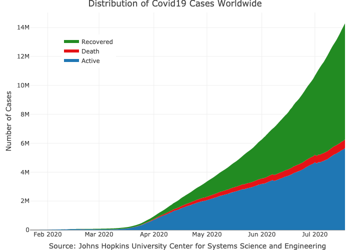
Plot the confirmed cases distribution by counrty with treemap plot:
conf_df <- coronavirus %>%
  filter(type == "confirmed") %>%
  group_by(country) %>%
  summarise(total_cases = sum(cases)) %>%
  arrange(-total_cases) %>%
  mutate(parents = "Confirmed") %>%
  ungroup()

  plot_ly(data = conf_df,
          type= "treemap",
          values = ~total_cases,
          labels= ~ country,
          parents=  ~parents,
          domain = list(column=0),
          name = "Confirmed",
          textinfo="label+value+percent parent")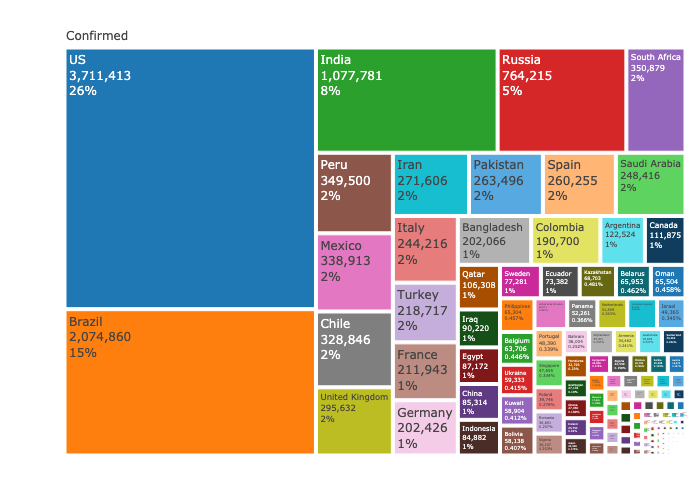
The raw data pulled and arranged by the Johns Hopkins University Center for Systems Science and Engineering (JHU CCSE) from the following resources: