![]()

![]()
![]()
biscale implements a set of functions for bivariate thematic mapping based on the tutorial written by Timo Grossenbacher and Angelo Zehr as well as a set of bivariate mapping palettes from Joshua Stevens’s tutorial. The package currently supports two-by-two and three-by-three bivariate maps:
In addition to support for both two-by-two and three-by-three maps, the package also supports four methods for calculating breaks for bivariate maps.
In order to resolve a conflict between the tibble package and biscale, the sf package is now a required dependency as opposed to being a suggested dependency.
The development version contains a new function, bi_scale_color(), which replicates the bivariate mapping workflow for point and line data. We don’t have any sample data for it yet, but the workflow mapping point data looks like this:
# create classes
data <- bi_class(pointData, x = xvar, y = yvar, style = "quantile", dim = 3)

# create map
map <- ggplot() +
  geom_sf(data = pointData, mapping = aes(color = bi_class), show.legend = FALSE) +
  bi_scale_color(pal = "DkBlue", dim = 3) +
  bi_theme()
The creation of classes works the same way. The only difference is (a) the use of the color (or colour) argument in the aesthetic mapping for geom_sf() and the use of bi_scale_color() afterwards!
If you want to use a different palette with biscale plots, you can use the new bi_pal_manual() function to create the plot and then apply it to bi_scale_fill() or bi_scale_color() using the pal argument.
# create classes
data <- bi_class(pointData, x = xvar, y = yvar, style = "quantile", dim = 2)

# create custom palette
custom_pal <- bi_pal_manual(val_1_1 = "#E8E8E8", val_1_2 = "#73AE80", val_2_1 = "#6C83B5", val_2_2 = "#2A5A5B")

# create map
map <- ggplot() +
  geom_sf(data = pointData, mapping = aes(color = bi_class), show.legend = FALSE) +
  bi_scale_color(pal = custom_pal, dim = 3) +
bi_theme()You should check the sf package website and the areal package website for the latest details on installing dependencies for that package. Instructions vary significantly by operating system. For best results, have sf installed before you install biscale. Other dependencies, like dplyr, will be installed automatically with areal if they are not already present.
For Linux users, steps will vary based on the flavor being used. Our configuration file for Travis CI and its associated bash script should be useful in determining the necessary components to install.
Once sf is installed, the easiest way to get biscale is to install it from CRAN:
Alternatively, the development version of biscale can be accessed from GitHub with remotes:
Creating bivariate plots in the style described by Grossenbacher and Zehr requires a number of dependencies in addition to biscale - ggplot2 for plotting and sf for working with spatial objects in R. We’ll also use cowplot in these examples:
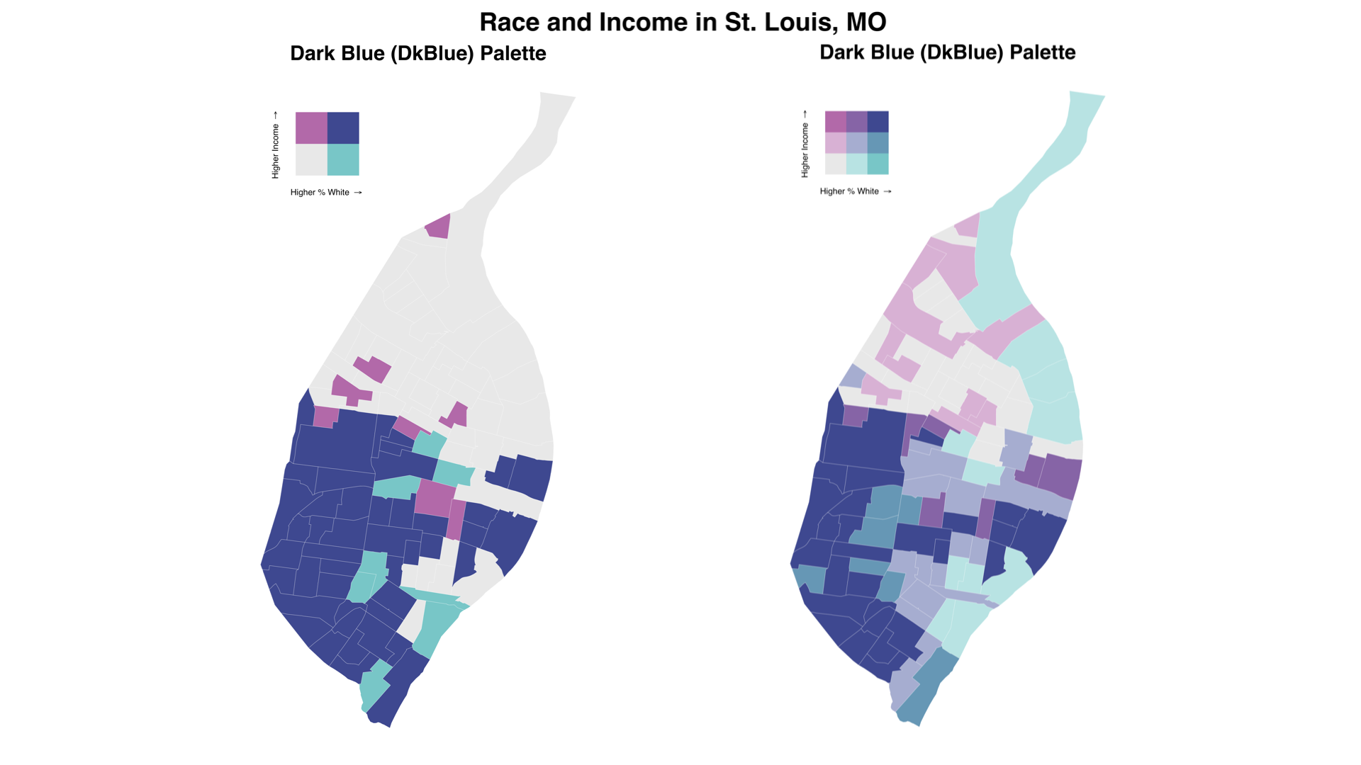
The biscale package comes with some sample data from St. Louis, MO that you can use to check out the bivariate mapping workflow. Our first step is to create our classes for bivariate mapping. biscale currently supports a both two-by-two and three-by-three tables of classes, created with the bi_class() function: :
# create classes
data <- bi_class(stl_race_income, x = pctWhite, y = medInc, style = "quantile", dim = 3)
The default method for calculating breaks is "quantile", which will provide breaks at 33.33% and 66.66% percent (i.e. tercile breaks) for three-by-three palettes. Other options are "equal", "fisher", and "jenks". These are specified with the optional style argument. The dim argument is used to adjust whether a two-by-two and three-by-three tables of classes is returned
Once breaks are created, we can use bi_scale_fill() as part of our ggplot() call:
# create map
map <- ggplot() +
  geom_sf(data = data, mapping = aes(fill = bi_class), color = "white", size = 0.1, show.legend = FALSE) +
  bi_scale_fill(pal = "DkBlue", dim = 3) +
  labs(
    title = "Race and Income in St. Louis, MO",
    subtitle = "Dark Blue (DkBlue) Palette"
  ) +
  bi_theme()
Other options for palettes include "Brown", "DkCyan", "DkViolet", and "GrPink". The bi_theme() function applies a simple theme without distracting elements, which is preferable given the already elevated complexity of a bivarite map. We need to specify the dimensions of the palette for bi_scale_fill() as well.
To add a legend to our map, we need to create a second ggplot object. We can use bi_legend() to accomplish this, which allows us to easily specify the fill palette, the x and y axis labels, and their size along with the dimensions of the palette:
legend <- bi_legend(pal = "DkBlue",
                    dim = 3,
                    xlab = "Higher % White ",
                    ylab = "Higher Income ",
                    size = 8)
Note that plotmath is used to draw the arrows since Unicode arrows are font dependent. This happens internally as part of bi_legend() - you don’t need to include them in your xlab and ylab arguments!
With our legend drawn, we can then combine the legend and the map with cowplot. The values needed for this stage will be subject to experimentation depending on the shape of the map itself.
# combine map with legend
finalPlot <- ggdraw() +
  draw_plot(map, 0, 0, 1, 1) +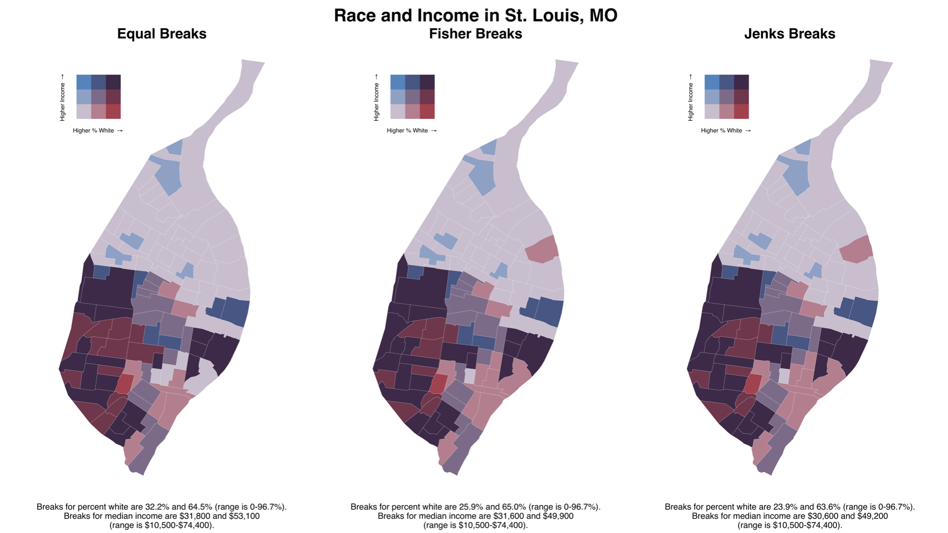
draw_plot(legend, 0.2, .65, 0.2, 0.2)The map at the top of the README uses the default "quantile" style for calculating breaks. The other options, "equal", "fisher", and "jenks", will produce narrower ranges for the percent white variable in particular:
In addition to the "DkBlue" palette show in the first map, there are a number of other options for palettes (including "Brown", which is not shown here) for two-by-two mapping:

These same options exist for three-by-three mapping as well:

All color palettes, including "Brown", can be previewed by using the bi_pal() function or by checking out that function’s documentation on the package website.
Please note that this project is released with a Contributor Code of Conduct. By participating in this project you agree to abide by its terms.