The SWIM package provides weights on simulated scenarios from a stochastic model, such that stressed model components (random variables) fulfil given probabilistic constraints (e.g. specified values for risk measures), under the new scenario weights. Scenario weights are selected by constrained minimisation of the relative entropy to the baseline model. The SWIM package is based on the paper Pesenti S.M, Millossovich P., Tsanakas A. (2019) “Reverse Sensitivity Testing: What does it take to break the model”.
The Vignette of the SWIM package is available in html format (https://utstat.toronto.edu/pesenti/SWIMVignette/) and as pdf(https://openaccess.city.ac.uk/id/eprint/23473/).
The SWIM package can be installed from CRAN :
alternatively from GitHub:
The SWIM package provides sensitivity analysis tools for stressing model components (random variables). Implemented stresses are:
| R functions | Stress |
|---|---|
stress() |
A wrapper for the stress_ functions |
stress_VaR() |
VaR risk measure, a quantile |
stress_VaR() |
VaR risk measure, a quantile |
stress_VaR_ES() |
VaR and ES risk measures |
stress_mean() |
means |
stress_mean_sd() |
means and standard deviations |
stress_moment() |
moments, functions of moments |
stress_prob() |
probabilities of intervals |
stress_user() |
user defined scenario weights |
Implemented functions allow to graphically display the change in the probability distributions under different stresses and the baseline model as well as calculating sensitivity measures.
Consider a portfolio Y = X1 + X2 + X3 + X4 + X5, where (X1, X2, X3, X4, X5) are correlated normally distributed with equal mean and different standard deviations. We stress the VaR (quantile) of the portfolio loss Y at levels 0.75 and 0.9 with an increase of 10%.
 # simulating the portfolio
set.seed(0)
SD <- c(70, 45, 50, 60, 75)
Corr <- matrix(rep(0.5, 5^2), nrow = 5) + diag(rep(1 - 0.5, 5))
x <- mvtnorm::rmvnorm(10^5,
   mean =  rep(100, 5),
   sigma = (SD %*% t(SD)) * Corr)
data <- data.frame(rowSums(x), x)
names(data) <- c("Y", "X1", "X2", "X3", "X4", "X5")
 # stressing the portfolio
rev.stress <- stress(type = "VaR", x = data,
   alpha = c(0.75, 0.9), q_ratio = 1.1, k = 1)
#> Stressed VaR specified was 722.9387 , stressed VaR achieved is 722.9378
#> Stressed VaR specified was 878.859 , stressed VaR achieved is 878.8296
Summary statistics of the baseline and the stressed model can be obtained via the summary() method.
#> $base
#>
#>
#>                     Y       X1       X2       X3       X4       X5
#> ------------  -------  -------  -------  -------  -------  -------
#> mean           500.18   100.14   100.01    99.93    99.98   100.13
#> sd             232.13    69.79    44.93    49.83    59.85    74.76
#> skewness         0.00    -0.01     0.00     0.01    -0.01     0.01
#> ex kurtosis     -0.04    -0.03    -0.02    -0.01    -0.02     0.00
#> 1st Qu.        342.56    53.24    69.70    66.23    59.45    49.72
#> Median         500.45   100.16   100.06   100.11   100.23    99.94
#> 3rd Qu.        657.22   147.33   130.31   133.51   140.33   150.80
#>
#> $`stress 1`
#>
#>
#>                     Y       X1       X2       X3       X4       X5
#> ------------  -------  -------  -------  -------  -------  -------
#> mean           534.03   108.20   104.85   105.38   106.70   108.89
#> sd             245.47    72.32    46.35    51.48    61.90    77.60
#> skewness        -0.06    -0.04    -0.03    -0.02    -0.04    -0.02
#> ex kurtosis     -0.29    -0.13    -0.10    -0.10    -0.12    -0.11
#> 1st Qu.        361.73    58.81    73.38    70.21    64.41    55.97
#> Median         532.15   108.59   105.08   105.65   107.33   109.02
#> 3rd Qu.        722.94   158.24   136.71   140.66   149.34   162.58
#>
#> $`stress 2`
#>
#>
#>                     Y       X1       X2       X3       X4       X5
#> ------------  -------  -------  -------  -------  -------  -------
#> mean           524.20   105.87   103.44   103.82   104.75   106.33
#> sd             249.62    73.14    46.81    52.01    62.57    78.46
#> skewness         0.09     0.04     0.04     0.05     0.04     0.06
#> ex kurtosis     -0.19    -0.09    -0.06    -0.06    -0.08    -0.07
#> 1st Qu.        352.14    55.99    71.60    68.34    62.00    52.93
#> Median         516.03   104.72   102.95   103.26   104.12   104.94
#> 3rd Qu.        687.58   155.33   134.95   138.82   146.79   159.24
Visual display of the change of empirical distribution functions of the portfolio loss Y from the baseline to the two stressed models.
plot_cdf(object = rev.stress, xCol = 1, base = TRUE)
#> Warning: Computation failed in `stat_ecdf()`:
#> there is no package called 'spatstat'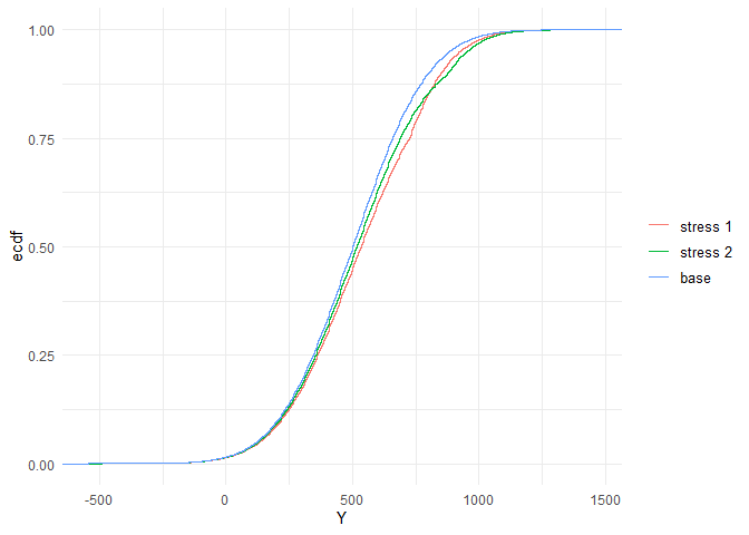
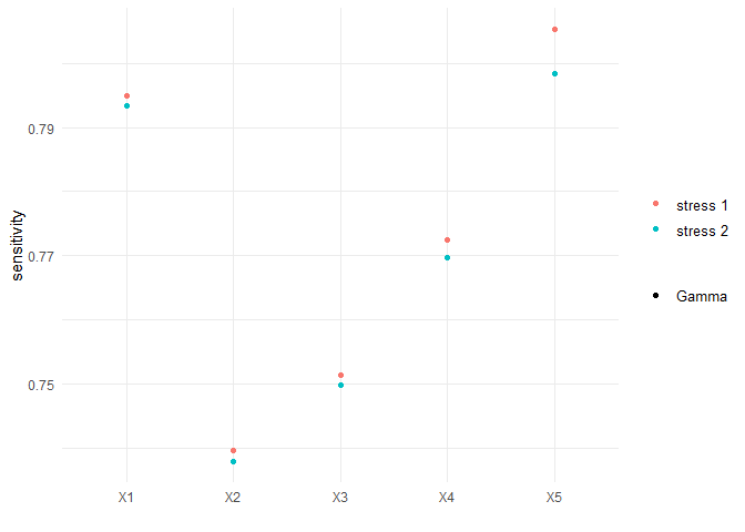
Sensitivity measures allow to assess the importance of the input components. Implemented sensitivity measures are the Kolmogorov distance, the Wasserstein distance and Gamma. Gamma, the Reverse Sensitivity Measure, defined for model component Xi, i = 1, …, 5, and scenario weights w by
Gamma = ( E(Xi * w) - E(Xi) ) / c,
where c is a normalisation constant such that |Gamma| <= 1, see https://doi.org/10.1016/j.ejor.2018.10.003. Loosely speaking, the Reverse Sensitivity Measure is the normalised difference between the first moment of the stressed and the baseline distributions of Xi.
| stress | type | Y | X1 | X2 | X3 | X4 | X5 |
|---|---|---|---|---|---|---|---|
| stress 1 | Gamma | 1.00 | 0.79 | 0.74 | 0.75 | 0.77 | 0.81 |
| stress 2 | Gamma | 1.00 | 0.79 | 0.74 | 0.75 | 0.77 | 0.80 |
| stress 1 | Kolmogorov | 0.00 | 0.00 | 0.00 | 0.00 | 0.00 | 0.00 |
| stress 2 | Kolmogorov | 0.00 | 0.00 | 0.00 | 0.00 | 0.00 | 0.00 |
| stress 1 | Wasserstein | 0.25 | 0.08 | 0.05 | 0.05 | 0.06 | 0.08 |
| stress 2 | Wasserstein | 0.14 | 0.04 | 0.03 | 0.03 | 0.04 | 0.04 |
Sensitivity to all sub-portfolios, (Xi + Xj), i,j = 1, …, 6:
 # sub-portfolios
f <- rep(list(function(x)x[1] + x[2]), 10)
k <- list(c(2, 3), c(2, 4), c(2, 5), c(2, 6), c(3, 4), c(3, 5), c(3, 6), c(4, 5), c(4, 6), c(5, 6))
importance_rank(rev.stress, xCol = NULL, wCol = 1, type = "Gamma", f = f, k = k)
#>     stress  type f1 f2 f3 f4 f5 f6 f7 f8 f9 f10
#> 1 stress 1 Gamma  7  6  3  1 10  9  5  8  4   2
Ranking the input components according to the chosen sensitivity measure, in this example using Gamma.
importance_rank(rev.stress, xCol = 2:6, type = "Gamma")
#> stress type X1 X2 X3 X4 X5
#> 1 stress 1 Gamma 2 5 4 3 1
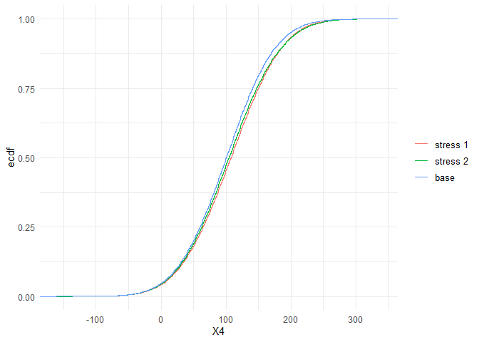
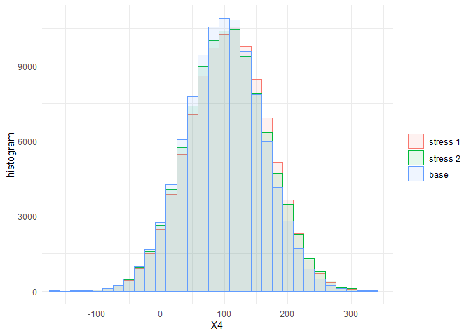
#> 2 stress 2 Gamma 2 5 4 3 1Visual display of the change of empirical distribution functions and density from the baseline to the two stressed models of X5, the portfolio component with the largest sensitivity. Stressing the portfolio loss Y, results in a distribution function of X5 that has a heavier tail.
plot_cdf(object = rev.stress, xCol = 5, base = TRUE)
#> Warning: Computation failed in `stat_ecdf()`:
#> there is no package called 'spatstat'