README

The package JointAI provides joint analysis and imputation of (generalized) linear regression models, (generalized) linear mixed models and parametric (Weibull) survival models with incomplete (covariate) data in the Bayesian framework.

The package performs some preprocessing of the data and creates a JAGS model, which will then automatically be passed to JAGS with the help of the R package rjags.

Installation

# install.packages("devtools")
devtools::install_github("NErler/JointAI")

Main functions

lm_imp()      # linear regression
glm_imp()     # generalized linear regression 
clm_imp()     # cumulative logit model
lme_imp()     # linear mixed model
glme_imp()    # generalized linear mixed model
clmm_imp()    # cumulative logit mixed model
survreg_imp() # parametric (Weibull) survival model
coxph_imp()   # Cox proportional hazards survival model

The functions lm_imp(), glm_imp() and clm_imp() use specification similar to their complete data counterparts lm() and glm() from base R and clm() from the package ordinal.

The functions for mixed models, lme_imp(), glme_imp() and clmm_imp() use similar specification as lme() from the package nlme (and clmm2() from ordinal).

survreg_imp() and coxph_imp() are missing data versions of survreg() and coxph() from the package survival.

Functions summary(), coef(), traceplot() and densityplot() provide a summary of the posterior distribution and its visualization.

GR_crit() and MC_error() provide the Gelman-Rubin diagnostic for convergence and the Monte Carlo error of the MCMC sample, respectively.

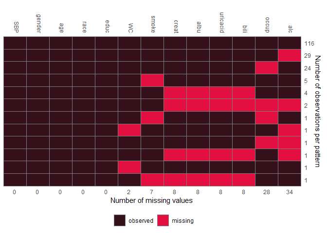
JointAI also provides functions for exploration of the distribution of the data and missing values, export of imputed values and prediction.

Minimal Example

Visualize the observed data and missing data pattern

library(JointAI)

op <- par(mar = c(2.5, 3, 2.5, 1), mgp = c(2, 0.8, 0))
plot_all(NHANES[c(1, 5:6, 8:12)], fill = '#e30f41', border = '#34111b', ncol = 4, nclass = 30)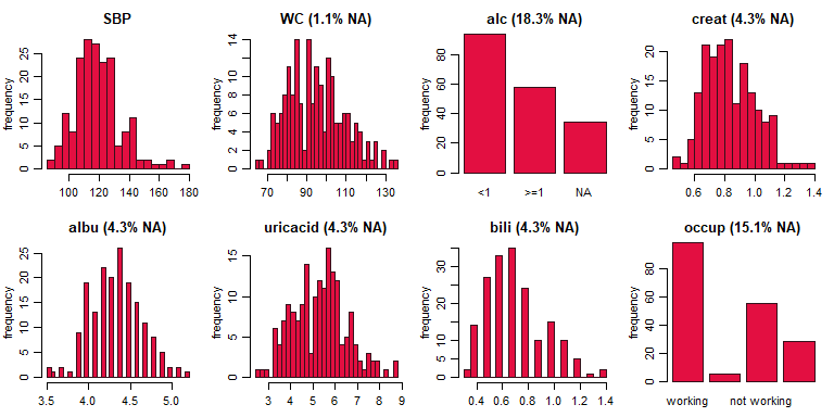

md_pattern(NHANES, color = c('#34111b', '#e30f41'))

Fit a linear regression model with incomplete covariates

lm1 <- lm_imp(SBP ~ gender + age + WC + alc + educ + bili,
              data = NHANES, n.iter = 500, progress.bar = 'none')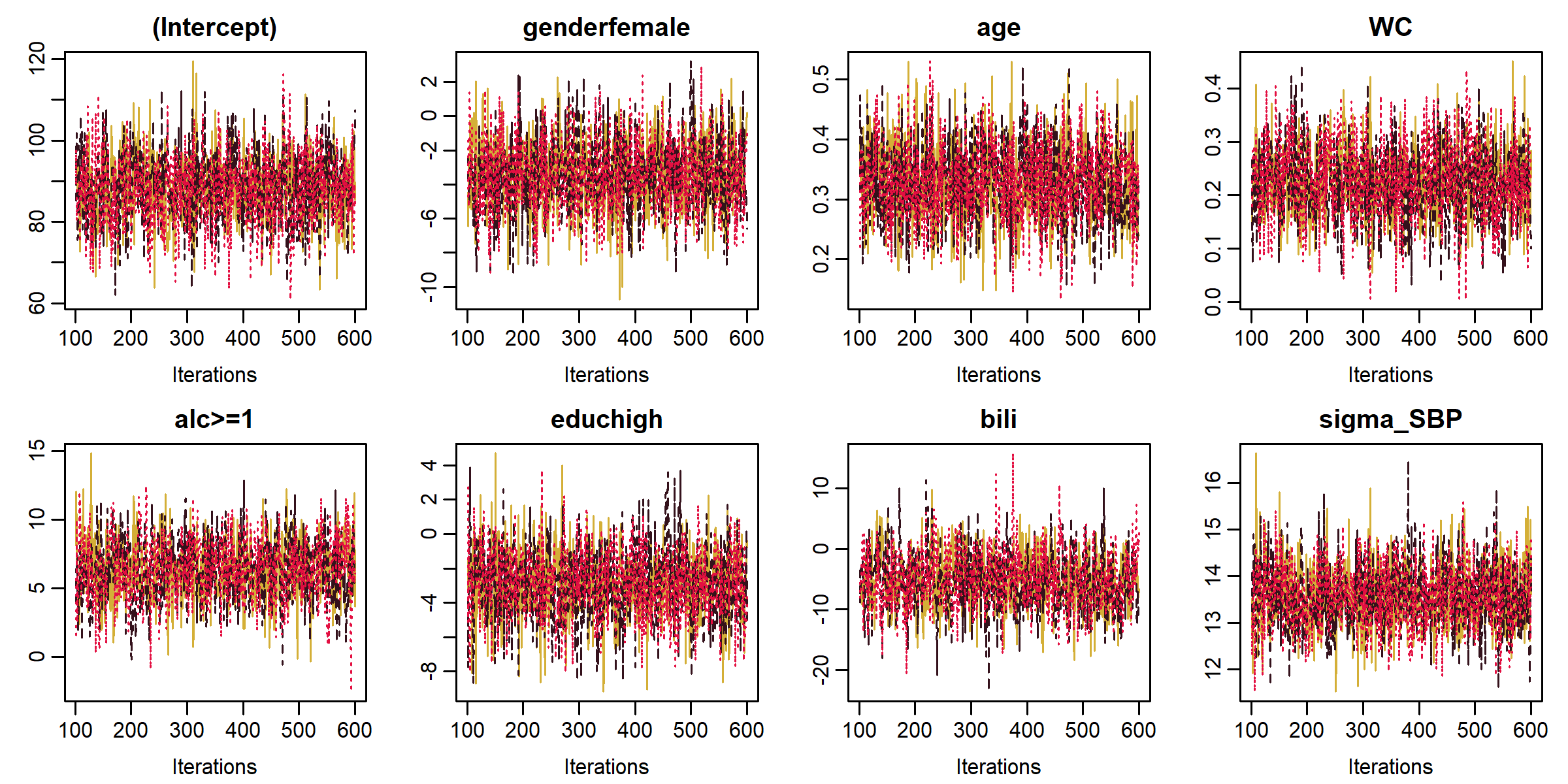

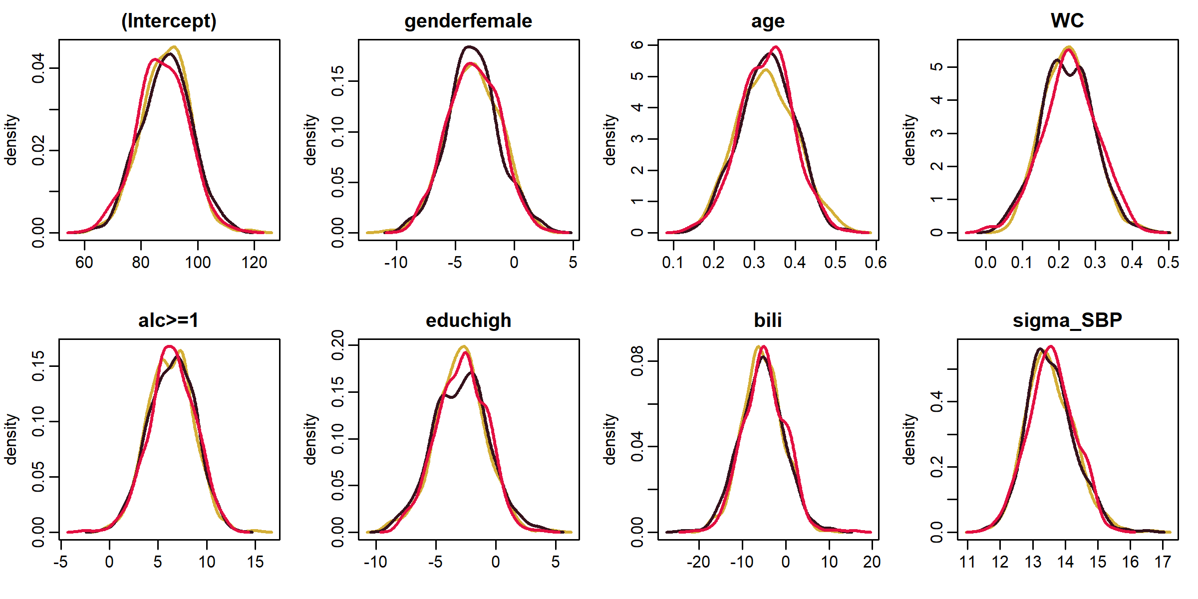
Visualize the MCMC sample

traceplot(lm1, col = c('#d4af37', '#34111b', '#e30f41'), ncol = 4)

densplot(lm1, col = c('#d4af37', '#34111b', '#e30f41'), ncol = 4, lwd = 2)

Summarize the Result

summary(lm1)
#> 
#>  Linear model fitted with JointAI 
#> 
#> Call:
#> lm_imp(formula = SBP ~ gender + age + WC + alc + educ + bili, 
#>     data = NHANES, n.iter = 500, progress.bar = "none")
#> 
#> Posterior summary:
#>                Mean     SD     2.5%   97.5% tail-prob. GR-crit
#> (Intercept)  88.330 8.7956  70.8815 105.510      0.000    1.02
#> genderfemale -3.439 2.2033  -7.8477   0.948      0.123    1.00
#> age           0.330 0.0682   0.2004   0.463      0.000    1.00
#> WC            0.225 0.0717   0.0865   0.364      0.000    1.01
#> alc>=1        6.388 2.3306   1.9035  10.788      0.008    1.00
#> educhigh     -2.908 2.1390  -7.3109   1.166      0.177    1.00
#> bili         -5.192 4.8641 -14.7564   3.913      0.289    1.01
#> 
#> Posterior summary of residual std. deviation:
#>           Mean    SD 2.5% 97.5% GR-crit
#> sigma_SBP 13.6 0.722 12.2    15       1
#> 
#> 
#> MCMC settings:
#> Iterations = 101:600
#> Sample size per chain = 500 
#> Thinning interval = 1 
#> Number of chains = 3 
#> 
#> Number of observations: 186

coef(lm1)
#>  (Intercept) genderfemale          age           WC       alc>=1     educhigh 
#>   88.3300380   -3.4387701    0.3298298    0.2253663    6.3883253   -2.9079009 
#>         bili 
#>   -5.1915762

confint(lm1)
#>                     2.5%       97.5%
#> (Intercept)   70.8814968 105.5095036
#> genderfemale  -7.8476897   0.9479861
#> age            0.2003926   0.4626324
#> WC             0.0865418   0.3641664
#> alc>=1         1.9034962  10.7884149
#> educhigh      -7.3109043   1.1658549
#> bili         -14.7563735   3.9129268
#> sigma_SBP     12.2366034  15.0167016