README

This package is the newer version of the older CMFunnels package. Development work will focus on this package from now on

It draws funnel plots using ggplot2 and allows users to specify whether they want ‘overdispersed’ limits, setting a Winsorisation percentage (default 10%)

This uses a log-transformation and truncation of the distribution for calculating overdispersion, whereas Spiegelhalter’s methods use a square-root and Winsorisation.

This package was originally developed for use in CM’s PhD project, but published on github in case it’s of use for others.

Please note that the ‘FunnelPlotR’ project is released with a Contributor Code of Conduct. By contributing to this project, you agree to abide by its terms.

Installation

install.packages("FunnelPlotR")
# or
remotes::install_github("https://github.com/chrismainey/FunnelPlotR")

Summary of Use

We will load the medpar dataset from Hilbe’s COUNT package. This is based on 1991 Medicare files for the state of Arizona (Hilbe, Joseph M (2014), Modeling Count Data, Cambridge University Press). We will first load the data and build a simple predictive model using a Poisson GLM.

library(FunnelPlotR)
library(COUNT)
library(ggplot2)

# lets use the 'medpar' dataset from the 'COUNT' package. Little reformatting needed
data(medpar)
medpar$provnum<-factor(medpar$provnum)
medpar$los<-as.numeric(medpar$los)

mod<- glm(los ~ hmo + died + age80 + factor(type), family="poisson", data=medpar)
summary(mod)
#> 
#> Call:
#> glm(formula = los ~ hmo + died + age80 + factor(type), family = "poisson", 
#>     data = medpar)
#> 
#> Deviance Residuals: 
#>     Min       1Q   Median       3Q      Max  
#> -5.7309  -1.9554  -0.5529   0.9717  14.5487  
#> 
#> Coefficients:
#>               Estimate Std. Error z value Pr(>|z|)    
#> (Intercept)    2.26875    0.01246 182.011  < 2e-16 ***
#> hmo           -0.07637    0.02393  -3.192  0.00142 ** 
#> died          -0.24574    0.01826 -13.458  < 2e-16 ***
#> age80         -0.02141    0.02050  -1.045  0.29617    
#> factor(type)2  0.24921    0.02099  11.871  < 2e-16 ***
#> factor(type)3  0.74869    0.02627  28.496  < 2e-16 ***
#> ---
#> Signif. codes:  0 '***' 0.001 '**' 0.01 '*' 0.05 '.' 0.1 ' ' 1
#> 
#> (Dispersion parameter for poisson family taken to be 1)
#> 
#>     Null deviance: 8901.1  on 1494  degrees of freedom
#> Residual deviance: 7977.7  on 1489  degrees of freedom
#> AIC: 13705
#> 
#> Number of Fisher Scoring iterations: 5

Now we have a regression that we can use to get a predicted los that we will compare to observed los:

medpar$prds<- predict(mod, type="response")

We can build a funnel plot object with standard Poisson limits, and outliers labelled.

a<-funnel_plot(numerator=medpar$los, denominator=medpar$prds, group = medpar$provnum, 
            title = 'Length of Stay Funnel plot for `medpar` data', Poisson_limits = TRUE,
            OD_adjust = FALSE,label_outliers = TRUE, return_elements = "plot")
a
#> $plot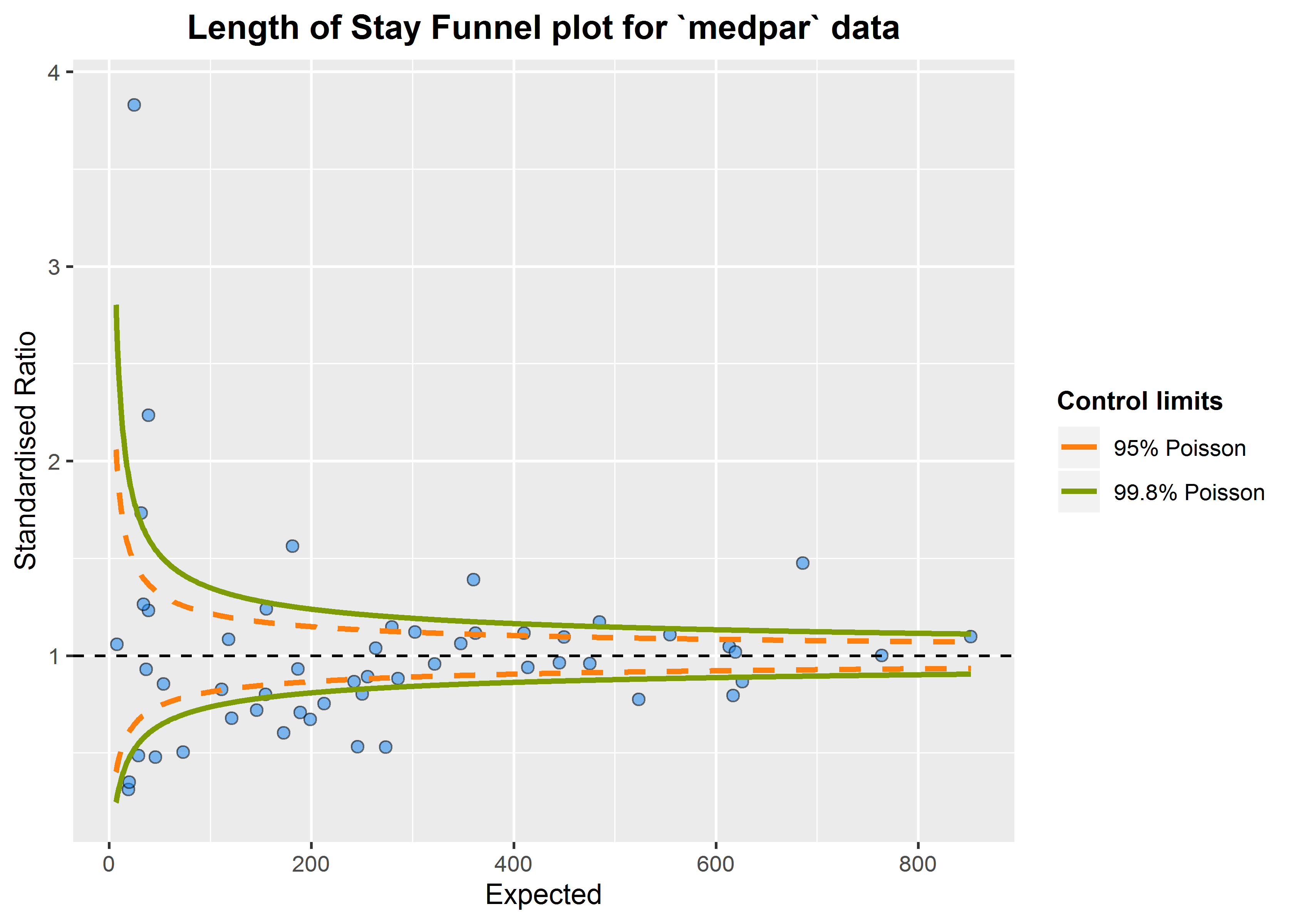

That looks like too many outliers! There is more variation in our data than we would expect, and this is referred to as: overdispersion. So lets check for it:
The following ratio should be 1 if our data are conforming to Poisson distribution assumption (conditional mean = variance). If it is greater than 1, we have overdispersion:


sum(mod$weights * mod$residuals^2)/mod$df.residual
#> [1] 6.240519

This suggest the variance is 6.24 times the condition mean, and definitely overdispersed. This is a huge topic, but applying overdispersed limits using either SHMI or Spiegelhalter methods adjust for this by inflating the limits:

b<-funnel_plot(numerator=medpar$los, denominator=medpar$prds, group = medpar$provnum, 
            title = 'Length of Stay Funnel plot for `medpar` data', Poisson_limits = FALSE,
            OD_adjust = TRUE, method = "SHMI",label_outliers = TRUE, return_elements = "plot")

b
#> $plot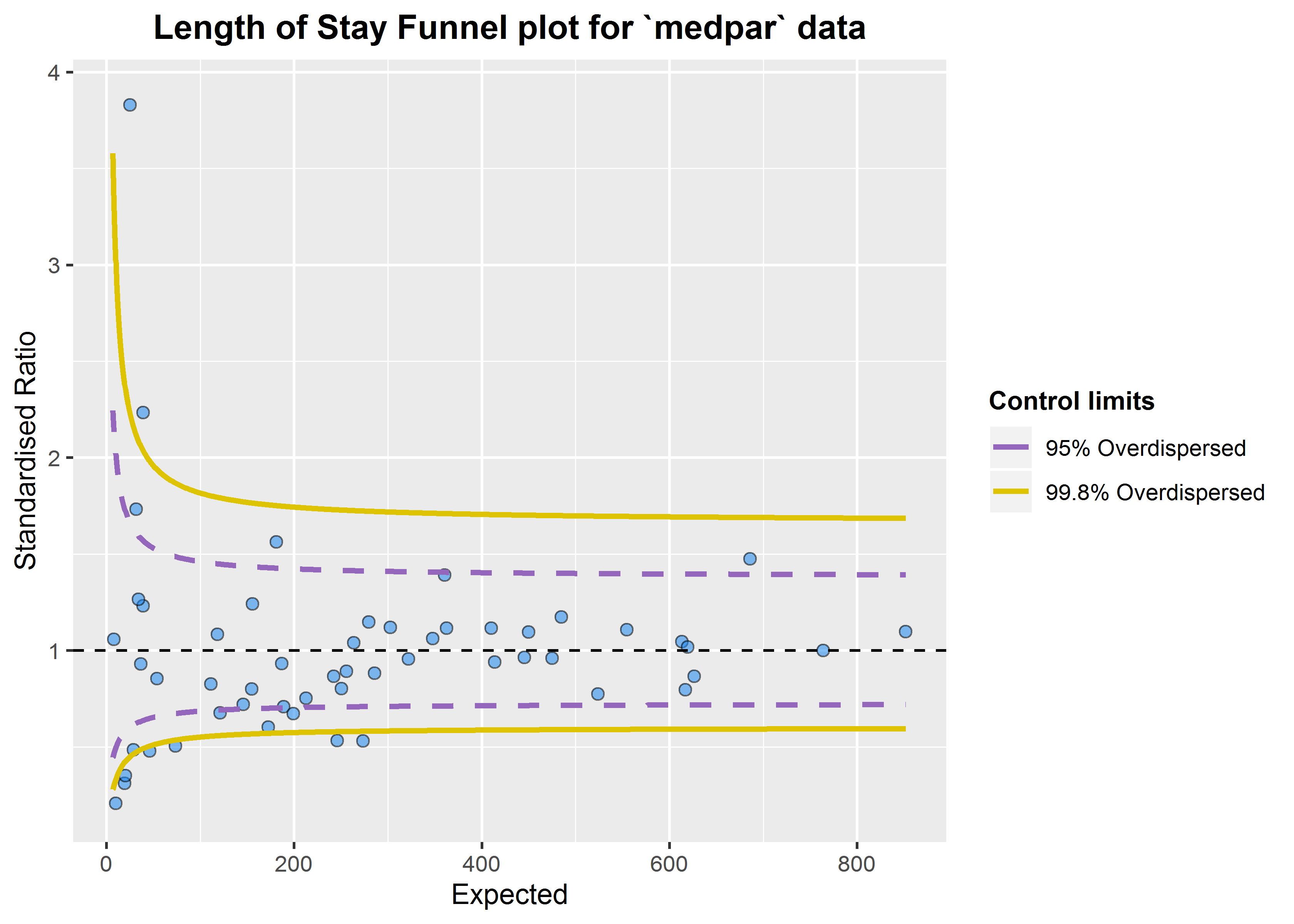

These methods can be used for any similar indicators, e.g. standardised mortality ratios, readmissions etc.

Funnel plots for risk-adjusted indicators

Funnel Plots

Installation

Summary of Use