
The EFAtools package provides functions to perform exploratory factor analysis (EFA) procedures and compare their solutions. The goal is to provide state-of-the-art factor retention methods and a high degree of flexibility in the EFA procedures. This way, implementations from R psych and SPSS can be compared. Moreover, functions for Schmid-Leiman transformation, and computation of omegas are provided. To speed up the analyses, some of the iterative procedures like principal axis factoring (PAF) are implemented in C++.
You can install the release version from CRAN with:
You can install the development version from GitHub with:
To also build the vignette when installing the development version, use:
Here are a few examples on how to perform the analyses with the different types and how to compare the results using the COMPARE function. For more details, see the vignette by running vignette("EFAtools", package = "EFAtools"). The vignette provides a high-level introduction into the functionalities of the package.
# load the package
library(EFAtools)

# Run all possible factor retention methods
N_FACTORS(test_models$baseline$cormat, N = 500, method = "ML")
#> Warning in N_FACTORS(test_models$baseline$cormat, N = 500, method = "ML"): ! 'x' was a correlation matrix but CD needs raw data. Skipping CD.
#>
#> ── Tests for the suitability of the data for factor a
#>
#> Bartlett's test of sphericity
#>
#> ✓ The Bartlett's test of sphericity was significant at an alpha level of .05.
#>   These data are probably suitable for factor analysis.
#>
#>   𝜒²(153) = 2173.28, p = 0
#>
#> Kaiser-Meyer-Olkin criterion (KMO)
#>
#> ✓ The overall KMO value for your data is marvellous with 0.916.
#>   These data are probably suitable for factor analysis.
#>
#> ── Number of factors suggested by the different facto
#>
#> ◌ Comparison data: NA
#> ◌ Empirical Kaiser criterion: 2
#> ◌ Hull method with CAF: 3
#> ◌ Hull method with CFI: 1
#> ◌ Hull method with RMSEA: 1
#> ◌ Kaiser-Guttman criterion with PCA: 3
#> ◌ Kaiser-Guttman criterion with SMC: 1
#> ◌ Kaiser-Guttman criterion with EFA: 1
#> ◌ Parallel analysis with PCA: 3
#> ◌ Parallel analysis with SMC: 3
#> ◌ Parallel analysis with EFA: 6
#> ◌ Sequential 𝜒² model tests: 3
#> ◌ Lower bound of RMSEA 90% confidence interval: 2
#> ◌ Akaike Information Criterion: 3

# A type SPSS EFA to mimick the SPSS implementation with
# promax rotation
EFA_SPSS <- EFA(test_models$baseline$cormat, n_factors = 3, type = "SPSS",
                  rotation = "promax")

# look at solution
EFA_SPSS
#>
#> EFA performed with type = 'SPSS', method = 'PAF', and rotation = 'promax'.
#>
#> ── Rotated Loadings ─────────────────────────────────
#>
#>       F1      F2      F3
#> V1   -.048    .035    .613
#> V2   -.001    .067    .482
#> V3    .060    .056    .453
#> V4    .101   -.009    .551
#> V5    .157   -.018    .438
#> V6   -.072   -.049    .704
#> V7    .001    .533    .093
#> V8   -.016    .581    .030
#> V9    .038    .550   -.001
#> V10  -.022    .674   -.071
#> V11   .015    .356    .232
#> V12   .020    .651   -.010
#> V13   .614    .086   -.067
#> V14   .548   -.068    .088
#> V15   .561    .128   -.070
#> V16   .555   -.050    .091
#> V17   .664   -.037   -.027
#> V18   .555    .004    .050
#>
#> ── Factor Intercorrelations ─────────────────────────
#>
#>       F1      F2      F3
#> F1    1.000   0.617   0.648
#> F2    0.617   1.000   0.632
#> F3    0.648   0.632   1.000
#>
#> ── Variances Accounted for ──────────────────────────
#>
#>                       F1      F2      F3
#> SS loadings           4.907   0.757   0.643
#> Prop Tot Var          0.273   0.042   0.036
#> Cum Prop Tot Var      0.273   0.315   0.350
#> Prop Comm Var         0.778   0.120   0.102
#> Cum Prop Comm Var     0.778   0.898   1.000
#>
#> ── Model Fit ────────────────────────────────────────
#>
#> CAF: .50
#> df: 102

# A type psych EFA to mimick the psych::fa() implementation with
# promax rotation
EFA_psych <- EFA(test_models$baseline$cormat, n_factors = 3, type = "psych",
                  rotation = "promax")

# compare the type psych and type SPSS implementations
COMPARE(EFA_SPSS$rot_loadings, EFA_psych$rot_loadings,
        x_labels = c("SPSS", "psych"))
#> Mean [min, max] absolute difference:  0.0090 [ 0.0001,  0.0245]
#> Median absolute difference:  0.0095
#> Max decimals where all numbers are equal: 0
#> Minimum number of decimals provided: 17
#>
#>        F1      F2      F3
#> V1    0.0150  0.0142 -0.0195
#> V2    0.0109  0.0109 -0.0138
#> V3    0.0095  0.0103 -0.0119
#> V4    0.0118  0.0131 -0.0154
#> V5    0.0084  0.0105 -0.0109
#> V6    0.0183  0.0169 -0.0245
#> V7   -0.0026 -0.0017  0.0076
#> V8   -0.0043 -0.0035  0.0102
#> V9   -0.0055 -0.0040  0.0117
#> V10  -0.0075 -0.0066  0.0151
#> V11   0.0021  0.0029  0.0001
#> V12  -0.0064 -0.0050  0.0136
#> V13  -0.0109 -0.0019  0.0163
#> V14  -0.0049  0.0028  0.0070
#> V15  -0.0107 -0.0023  0.0161
#> V16  -0.0051  0.0028  0.0074
#> V17  -0.0096 -0.0001  0.0136
#> V18  -0.0066  0.0014  0.0098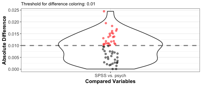
# Perform a Schmid-Leiman transformation
SL <- SL(EFA_psych)

# Compute omegas from the Schmid-Leiman solution
OMEGA(SL, factor_corres = rep(c(3, 2, 1), each = 6))
#> Omega total, omega hierarchical, and omega subscale for the general factor (top row) and the group factors:
#>
#>      tot  hier   sub
#> g  0.883 0.750 0.122
#> F1 0.769 0.501 0.268
#> F2 0.764 0.498 0.266
#> F3 0.745 0.536 0.209If you want to contribute or report bugs, please open an issue on GitHub or email us…